Week 3 - Solving second order ODEs

Aim: To simulate the motion of a damped pendulum and visualize its behavior using Python.

Objective: To understand the dynamics of a damped pendulum and observe its motion over time.

Problem Statement: To simulate the motion of a damped pendulum with given parameters and visualize its displacement, velocity, and trajectory.

Python Code:

import numpy as np
from scipy.integrate import odeint
import matplotlib.pyplot as plt
from matplotlib.patches import Rectangle
from matplotlib.animation import FuncAnimation

# Constants
g = 9.81   # gravity in m/s^2
L = 1.0    # length of the pendulum in m
m = 1      # mass of the ball in kg
b = 0.05   # damping coefficient
theta_0 = [0, 3]  # initial angular displacement and angular velocity
t = np.linspace(0, 20, 200)  # time array

# Function Definition
def model(theta, t, b, g, L, m):
    theta_1 = theta[0]
    theta_2 = theta[1]
    dtheta1_dt = theta_2
    dtheta2_dt = -(b / m) * theta_2 - (g / L) * np.sin(theta_1)
    dtheta_dt = [dtheta1_dt, dtheta2_dt]
    return dtheta_dt

# Calling the function
theta = odeint(model, theta_0, t, args=(b, g, L, m))

# Plotting displacement and velocity
plt.figure(figsize=(10, 6))
# Plot displacement
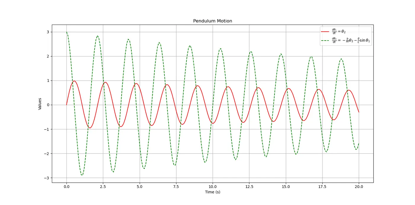
plt.plot(t, theta[:, 0], 'r-', label=r'$\frac{d\theta_1}{dt}=\theta_2$')
# Plot velocity
plt.plot(t, theta[:, 1], 'g--', label=r'$\frac{d\theta_2}{dt}=-\frac{b}{m}\theta_2-\frac{g}{L}\sin\theta_1$')
plt.title('Pendulum Motion')
plt.xlabel('Time (s)')
plt.ylabel('Values')
plt.legend(loc='best')
plt.grid(True)
plt.show()

# Function to update the animation at each frame
def update(frame):
    x = L * np.sin(theta[frame, 0])
    y = -L * np.cos(theta[frame, 0])
    pendulum.set_data([0, x], [0, y])
    trajectory.set_data(L * np.sin(theta[:frame, 0]), -L * np.cos(theta[:frame, 0]))
    return pendulum, trajectory, base, title, xlabel, ylabel

# Create a figure and axis for animation
fig, ax = plt.subplots()
ax.set_xlim(-1.5, 1.5)
ax.set_ylim(-1.5, 1.5)
ax.set_aspect('equal')
ax.grid()

# Plot the hinge point
ax.plot(0, 0, 'ko', markersize=5)

# Plot the base (wall)
base = Rectangle((-0.05, -0.1), 0.1, 0.2, color='gray')
ax.add_patch(base)

# Plot the trajectory
trajectory, = ax.plot([], [], 'b--', lw=1, alpha=0.5)

# Plot the pendulum
pendulum, = ax.plot([], [], 'ro-', lw=2)

# Add title
title = ax.text(0.5, 1.05, 'Pendulum Motion Animation', transform=ax.transAxes,
                ha='center', fontsize=12)

# Add axis labels
xlabel = ax.text(0.5, -0.1, 'x', transform=ax.transAxes,
                 ha='center', fontsize=10)
ylabel = ax.text(-0.15, 0.5, 'y', transform=ax.transAxes,
                 va='center', rotation='vertical', fontsize=10)

# Function to initialize the animation
def init():
    pendulum.set_data([], [])
    trajectory.set_data([], [])
    return pendulum, trajectory, base, title, xlabel, ylabel

# Create the animation
ani = FuncAnimation(fig, update, frames=len(theta), init_func=init, blit=True)

# Save the animation as a GIF
ani.save('pendulum_animation.gif', writer='pillow', fps=60)

plt.title('Pendulum Motion Animation')
plt.xlabel('x')
plt.ylabel('y')
plt.show()

Solution Procedure:

Defining Parameters:

• Initialize the constants such as gravity (g), length of the pendulum (L), mass of the ball (m), damping coefficient (b), initial angular displacement (theta_0), and time array (t).

Modeling the Pendulum Motion:

• Define a function (model) representing the differential equations governing the motion of the damped pendulum.
• Use odeint from scipy.integrate to solve the differential equations and obtain the angular displacement and velocity over time.
• Plotting Displacement and Velocity:
• Plot the angular displacement and velocity against time using matplotlib.pyplot.
• Add appropriate labels, legends, and grid to enhance readability.

Animating the Pendulum Motion:

• Create an animation of the pendulum motion using matplotlib.animation.FuncAnimation.
• Define functions to update the pendulum's position at each frame (update) and to initialize the animation (init).
• Add visual elements such as the hinge point, base (wall), and trajectory to enhance the animation.

Visualizing Results & Discussion:

• Visualize the displacement, velocity, and trajectory of the pendulum motion.
• Discuss the behavior observed in the plots and animation, such as the damping effect on the pendulum's motion and the influence of initial conditions and parameters.

Results & Discussion:

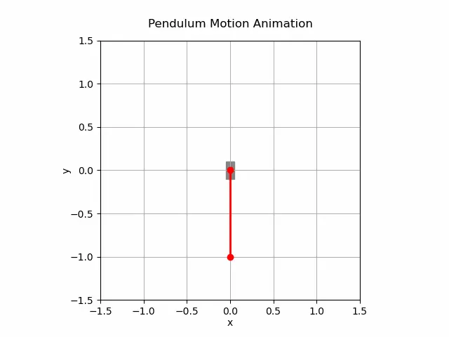
The simulation and visualization of the damped pendulum motion provide valuable insights into its behavior. The plots of displacement and velocity demonstrate how the pendulum's motion evolves over time. The animation vividly illustrates the swinging motion of the pendulum, showcasing the damping effect and the trajectory followed by the pendulum's bob.

Conclusion:

• In this simulation of a pendulum motion, we explored the behavior of the system under different damping conditions. Initially, we observed the pendulum's motion with a relatively low damping coefficient, resulting in oscillations that gradually diminished over time. As the damping coefficient increased, we noticed a more pronounced damping effect, causing the pendulum's oscillations to "die down" more rapidly.
• This die-down effect can be attributed to the increased energy dissipation within the system due to damping. Higher damping coefficients lead to greater energy loss, resulting in a quicker decay of the pendulum's oscillations. Consequently, the pendulum's motion converges towards equilibrium more rapidly, exhibiting less pronounced oscillations over time.
• By adjusting the damping coefficient, we can control the rate at which the pendulum's motion diminishes, allowing for a deeper understanding of the interplay between damping and oscillatory behavior in mechanical systems.