Week 3 - Solving second order ODEs

AIM: To write a program that solves the following ODE.

Description:

In Engineering, ODE is used to describe the transient behavior of a system. A simple example is a pendulum

The way the pendulum moves depends on the Newtons second law. When this law is written down, we get a second order Ordinary Differential Equation that describes the position of the "ball" w.r.t time.

Similarly, there are hundreds of ODEs that describe key phenomena and if you have the ability to solve these equations then you will be able to simulate any of theses systems.

In the above equation,

g = gravity in m/s2,

L = length of the pendulum in m,

m = mass of the ball in kg,

b=damping coefficient.

Write a program in Python that will simulate the pendulum motion, just like the one shown in the start of this challenge.

use,

L=1 metre,

m=1 kg,

b=0.05.

g=9.81 m/s2.

CASE 1:

• For integrating the ODE we need to define a system which is our model which we defined already.
• Then we need to define initial conditions, time arrays and arguments.
• Here, theta_0 is our initial condition for our angle.
• Model is a function which define ODE as a system.
• We use ODEINT to solve our differential equation.
• Two differential equations are defined as adtheta1_dt and dtheta2_dt.
• And then the 2 equations are combined as dtheta_dt.
• And then return the value of dtheta_dt.
• Theta is our final solution and then plot the results.
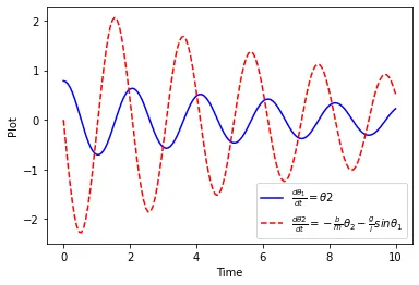
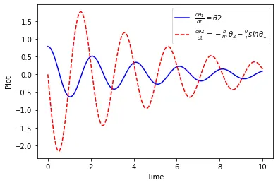
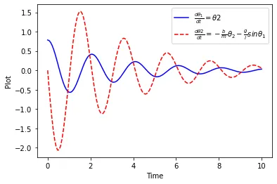
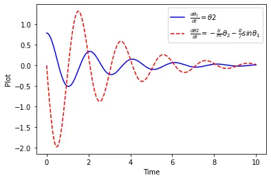
• Here theta1 is a angular displacement and theta2 is a angular velocity.
• For different values of b;

for b = 0.002

for b = 0.004

for b = 0.006

for b = 0.008

for b = 0.1

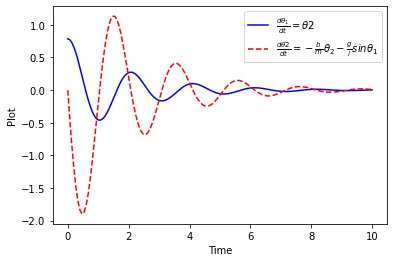
From the figures depicted above, it can be concluded that as the damping coefficient increases, the angular velocity and the angular displacement decreases.

Python code for Case 1

import numpy as np
from scipy.integrate import odeint
import matplotlib.pyplot  as plt
import math

# Function that return dz/dt
def model (theta, t, b, g, l, m):
    theta1 = theta[0]
    theta2 = theta[1]
    dtheta1_dt = theta2
    dtheta2_dt = -(b/m)*theta2 - (g/l)*math.sin(theta1)
    dtheta_dt = [dtheta1_dt, dtheta2_dt]
    return dtheta_dt

# Inputs
b = 0.1
g = 9.81
l = 1
m = 0.1

# Initial Conditions
theta_0 = [math.pi/4, 0]
 
# Time points
t = np.linspace(0,10,150)

#Solving ODE
theta = odeint(model, theta_0, t, args = (b,g,l,m))
 
# Plot
plt.plot(t, theta[:,0],'b-',label = r'$\frac{d\theta_1}{dt} =\theta2$')
plt.plot(t, theta[:,1],'r--',label = r'$\frac{d\theta2}{dt}=-\frac{b}{m}\theta_2-\frac{g}{l}sin\theta_1$')
plt.xlabel('Time')
plt.ylabel('Plot')
plt.legend(loc= 'best')
plt.show()

CASE 2:

Animation;

for animation we have used the linspace command to get 150 images,

Python code for Case 2:

import numpy as np
from scipy.integrate import odeint
import matplotlib.pyplot  as plt
import math

# Function that return dz/dt
def model (theta, t, b, g, l, m):
    theta1 = theta[0]
    theta2 = theta[1]
    dtheta1_dt = theta2
    dtheta2_dt = -(b/m)*theta2 - (g/l)*math.sin(theta1)
    dtheta_dt = [dtheta1_dt, dtheta2_dt]
    return dtheta_dt

# Inputs
b = 0.002
g = 9.81
l = 1
m = 0.1
ct = 1

# Initial Conditions
theta_0 = [math.pi/2, 0]
 
# Time points
t = np.linspace(0,10,150)

#Solving ODE
theta = odeint(model, theta_0, t, args = (b,g,l,m))
x1 = 0
y1 = 0

# all the angular displacement and zero angular velocity
for ang in theta[:,0]:   
   x2 = l*math.sin(ang)
   y2 = -l*math.cos(ang)

	# saveing images in png format
   filename = str(ct) + ".png"
   ct = ct + 1
    
    # Plot
   plt.figure()
   plt.plot([-1.5,1.5],[0,0],linewidth=8)
   plt.plot([x1,x2],[y1,y2],linewidth=3)
   plt.plot(x2,y2,"o",markersize=15)
   plt.xlim([-1.5,1.5])
   plt.ylim([-1.5,1.5])
   plt.savefig(filename)

GIF animation:

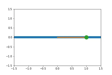
Here the image depicts real life condition of a pendulum. The bob is released from top and have a higher velocity and the dispalcement decreases as time increases.