Week 3 - Solving second order ODEs
Objective:
write a program that solve the given ODE.
code:
import math
import numpy as np
import matplotlib.pyplot as plt
from scipy.integrate import odeint
def system(theta_init,time,b,g,l,m):
theta_1 = theta_init[0]
theta_2 = theta_init[1]
dtheta1_dt = theta_2
dtheta2_dt = ((-b/m)*dtheta1_dt)-((g/l)*math.sin(theta_1))
dtheta_dt = [dtheta1_dt,dtheta2_dt]
return dtheta_dt
b = 0.05
g = 9.81
l = 1
m = 1
theta_init = [0,3]
time = np.linspace(0,20,200)
theta = odeint(system,theta_init,time,args=(b,g,l,m))
ang_disp = theta[:,0]
ang_vel = theta[:,1]
plt.figure(figsize=(10,6))
plt.plot(time,ang_disp,'b-',label='ANGULAR DISPLACEMENT')
plt.plot(time,ang_vel,'r-',label='ANGULAR VELOCITY')
plt.legend()
plt.xlabel('time')
plt.ylabel('displacement and velocity')
plt.title('Angular displacement and velocity of Simple Pendulum')
plt.grid()
plt.show()
Result:
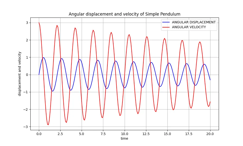
Resulted figure derived by solving the ODE using python code, y-axis shows the variation of displacement and velocity values over tiime (x-axis).tells that, pendulum reciprocates for 20secs. The bob has a angular velocity of 3rad/sec at time 0sec and radually reduces as time progress because of the damping effect given in the problem.
Objective:
This ODE represents the equation of motion of a simple pendulum with damping
import matplotlib.pyplot as plt
import numpy as np
from scipy.integrate import odeint
import math
b = 0.05
g = 9.81
l = 1
m = 1
theta_init = [0,3]
time = np.linspace(0,20,50)
def system(theta_init,time,b,g,l,m):
theta_1 = theta_init[0]
theta_2 = theta_init[1]
dtheta1_dt = theta_2
dtheta2_dt = ((-b/m)*dtheta1_dt)-((g/l)*math.sin(theta_1))
dtheta_dt = [dtheta1_dt,dtheta2_dt]
return dtheta_dt
theta = odeint(system,theta_init,time,args=(b,g,l,m))
ang_disp = theta[:,0]
x0=0
y0=0
ct = 1
for i in range(len(time)):
disp = ang_disp[i]
x1=1*(math.sin(disp))
y1=-1*(math.cos(disp))
filename = str(ct) + '.png'
ct = ct + 1
plt.figure()
plt.plot([-1,1],[0,0],'b')
plt.plot([x0,x1],[y0,y1],'g')
plt.plot(x1,y1,marker='o',color='r')
plt.xlim(-1.5,2)
plt.ylim(-1.5,1)
plt.savefig(filename)
Results:
The gif.file is attached with this solution.Please check the link to visualize the simple pendulum motion which is solved using ODE and executed by python code.