Week 3 - Solving second order ODEs
AIM:
Write a program in Python that will simulate the pendulum motion, just like the one shown in the start of this challenge.
use,
L=1 metre,
m=1 kg,
b=0.05.
g=9.81 m/s2.
Simulate the motion between 0-20 sec, for angular displacement=0,angular velocity=3 rad/sec at time t=0.
When you do this you will get the position of the pendulum as a function of time. Use this information to animate the motion of the pendulum, as shown in the below figure.
OBJECTIVE:
The second-order equation is nothing but a higher rank of the polynomial equation is 2. There are many second-order equations are in practice. A pendulum is one of the examples for it. Here a second-order equation is created and solved in python, creates plots for each position of a pendulum and animated using Magick.
CODE:
# Simulation of motion of pendulum
import math
import matplotlib.pyplot as plt
import numpy as np
from scipy.integrate import odeint
# function that return dz\\dt
def model(theta,t,b,g,l,m):
theta1 = theta [0]
theta2 = theta [1]
dtheta1_dt = theta2
dtheta2_dt = -(b/m)*theta2 - (g/l)*math.sin(theta1)
dtheta_dt = [dtheta1_dt,dtheta2_dt]
return dtheta_dt
# Input
b=0.05 # damping coefficient.
g=9.81 # gravity in m/s2
l=1 # length of the pendulum in m
m=0.1 # mass of the ball in kg
# Initial condition
theta_0 = [0,3]
# Time points
t = np.linspace(0,20,150)
# Solve ODE
theta = odeint(model,theta_0,t,args =(b,g,l,m))
# Plot
plt.plot(t,theta[:,0],\'b--\',label = r\'$\\frac{d\\theta_1}{dt} = \\theta2 $\')
plt.plot(t,theta[:,1],\'r--\',label = r\'$\\frac{d\\theta2}{dt} = -\\frac{b}{m}\\theta_2 -\\frac{g}{l}sin\\theta_1 $\')
plt.xlabel(\'Time\')
plt.ylabel(\'Plot\')
plt.xlim([0,12])
plt.legend(loc = \'best\')
plt.show()
# Animation
THETA3=[]
for theta3 in theta[:,0]:
THETA3.append(theta3)
ct=1
for THETA4 in THETA3:
x0=0
y0=0
x1=l*math.sin(THETA4)
y1=-l*math.cos(THETA4)
filename=\'Pendulum%05d.png\'%ct
ct=ct+1
plt.plot([-0.2,0.2],[0,0]) # Horizontal support or pendulum
plt.plot([x0,x1],[y0,y1]) # String of pendulum
plt.plot(x1,y1,\'-o\') # Bob tied at the end
plt.xlim([-1.5,1.5])
plt.ylim([-1.5,1])
plt.title(\'Motion of Pendulum\')
plt.savefig(filename)
plt.show()
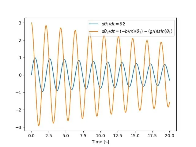
PLOTS FIGURE:
RESULTS:
Here second order differential equation is solved using python, and result animated using Magick. Using this equation pendulum animation created which reflects the pendulum position with respect to time.
YOUTUBE LINK:-https://youtu.be/w_hih7e1G5o