Week 4 - CHT Analysis on Exhaust port

Aim: Steady-state CHT analysis on Exhaust port at an inlet velocity of5m/sec

Objective: The objectives will mainly focus on

1. Give a brief description of why and where a CHT analysis is used.
2. Maintain the y+ value according to the turbulence model and justify the results.
3. Calculate the wall/surface heat transfer coefficient on the internal solid surface & show the velocity & temperature contours in appropriate areas.
4. How would you verify if the HTC predictions from the simulations are right? On what factors does the accuracy of the prediction depend?

Introduction: Conjugate heat transfer analysis is based on a mathematically structured problem, which describes the heat transfer between a body and a fluid flowing over or inside it as a result of interaction between two objects. At the matching interface, the details are provided for temperature distribution and heat flux along the interface eliminating the need of calculating the heat transfer coefficient. Moreover, the heat transfer coefficient can be calculated later.

One of the simplest ways to realize conjugation is through numerical methods. The boundary condition for the fluid and solid interface is set and solved through iteration methods. There are no right guesses for the values of the initial boundary condition for the convergence except through the hit and trial method.

Application: The conjugate heat transfer methods have become a more powerful tool for modeling and investigating nature phenomena and engineering systems in different areas ranging from aerospace and nuclear reactors to thermal goods treatment and food processing from the complex procedures in medicines to ocean thermal interaction in metrology.

CHT in recent years has significantly improved the cooling performance of electronic equipment such as the design of heat sinks and the design of heat exchangers for the waste treatment plant. One such application of CHT is the exhaust port system.

Solving and modeling approach

1. The exhaust port was modeled into the Spaceclaim.
2. The exhaust port is a three-dimensional model containing four inlets and one outlet. Despite having isothermal boundary conditions and a uniform flow rate at the four inlets, the model cannot be cut into two halves to save computational time because of its asymmetrical nature. Therefore the whole model is discretized and is considered for meshing.
3. CHT analysis requires both the solid and the liquid volume under consideration, Spaceclaim gives an option of volume extract for selecting edges for fluid volume.
4. Both the solid volume and liquid volume are copied into one component.
5. Share topology is created.
6. Spaceclaim gives an option for share coincident topology, when share coincident topology is selected and executed, the mesh from the fluid volume and the solid volume are said to be conformal with each other which is a requirement for CHT analysis.
7. The exhaust port is loaded into the meshing window and then simulated for baseline mesh and the refined mesh.
8. The named selections are created ( inlet, outlet, outer wall convection)
9. The necessary contour images and graphs are studied to understand the behavior of temperature, velocity, and surface heat transfer coefficient at the interface.

Pre-processing and solver setting

Baseline mesh

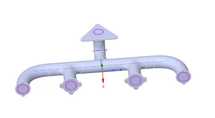
The geometry is loaded into Spaceclaim

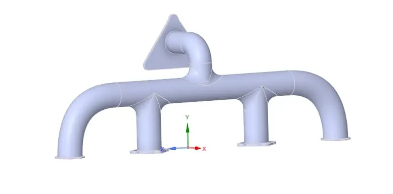
Fluid volume extraction

It is the process of extracting the fluid volume from the solid volume.

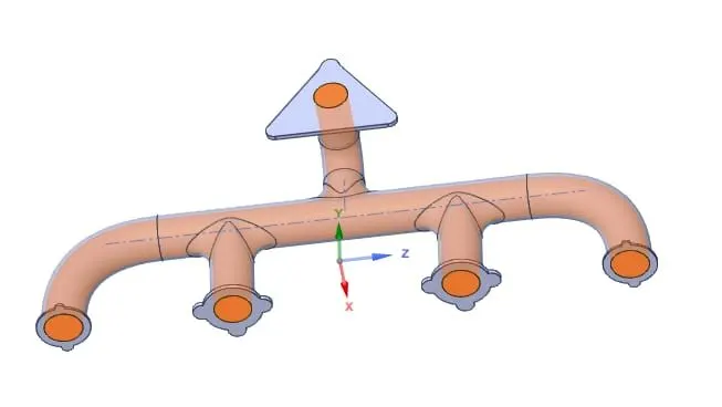
Share topology

It is the process of sharing information from fluid volume to solid volume. It plays important criteria in CHT analysis.

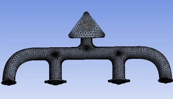
Meshing: It is the process of discretizing the geometry into a small number of volumes containing nodes. Since the geometry is complex and the mesh is unstructured therefore the finite volume scheme is used as a discretization scheme.

In this case, the default element size of ANSYS-FLUENT is used (0.15m).

MESH QUALITY

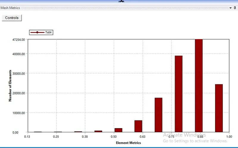
Mesh statistics

number of elements 135747

number of nodes 27104

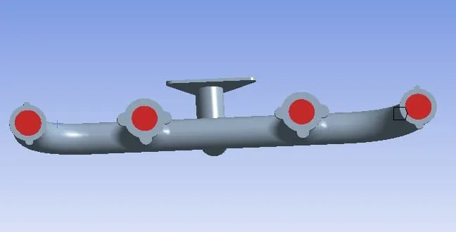
Named selection

inlet boundary condition(velocity inlet)@5m/sec

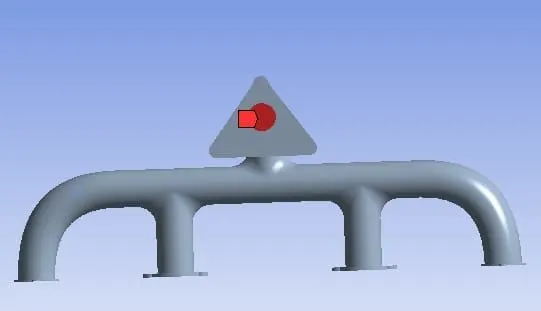
outlet(pressure oulet)Gauge pressure 0pa

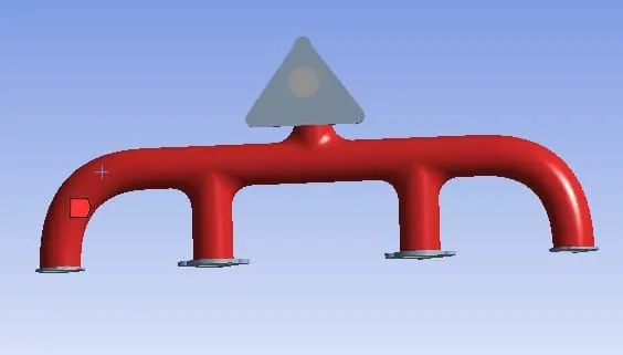
Outlet wall convection(Heat transfer coefficient 20W/m^2K free stream temperature 300K).

The flanges around the inlet and the component encompassing the outlet are adiabatic (no heat transfer takes place through these walls).

Setting up of physics and boundary conditions

The geometry orientation in the setup window. The blue-colored lines are inlet, and the red-colored lines are outlet.

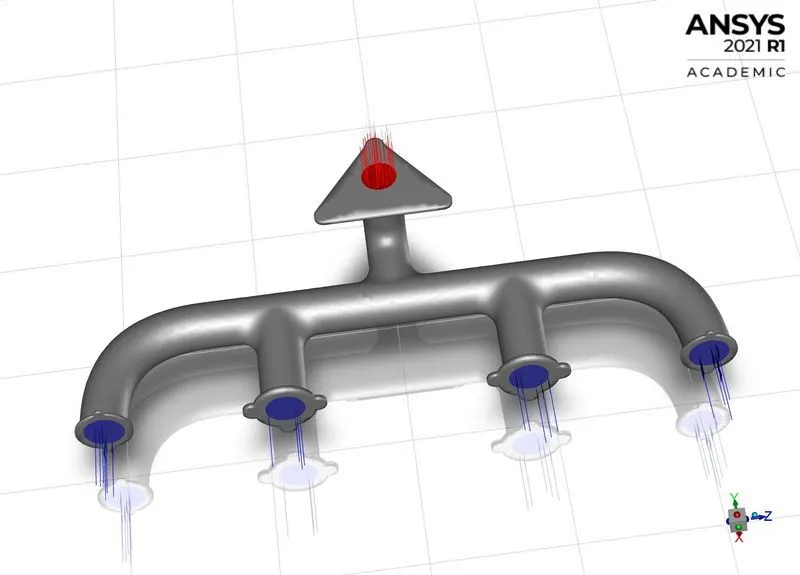
set up

The different boundary conditions are listed below

• Inlet boundary condition

1. Type:Velocity inlet
2. Velocity magnitude:5m/sec
3. temperature:700k

• Outlet boundary condition

1. Type:Pressure outlet
2. Gauge pressure:0pa

• outer wall convection

1. Type:wall
2. Thermal condition:convection
3. Heat transfer coefficient:20W/m^2k

The rest boundary condition values are set up as default values in ANSYS-FLUENT.

• Energy equation:It is turned on.
• viscous model:it is set to k-WSST

Material properties

fluid

• Material Name:Air
• Density:1.225kg/m^3
• specific heat:1006.43J/kgk
• Thermal conductivity:0.0242w/mk
• viscous:1.7894e - 05kg/m-sec

solid

• Material name:Aluminum
• specific heat:871J/kgk
• Thermal conductivity:202.4w/mk

simple method

Residual plot

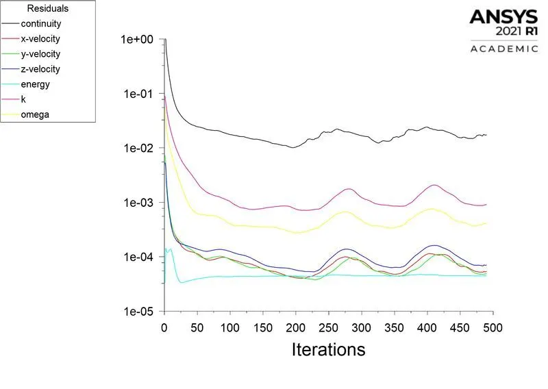
Surface heat transfer coefficient

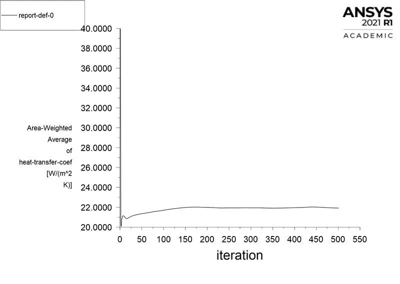
Surface heat transfer coefficient value:21.927121w/m^2k

SIMPLE METHOD

Residual plot

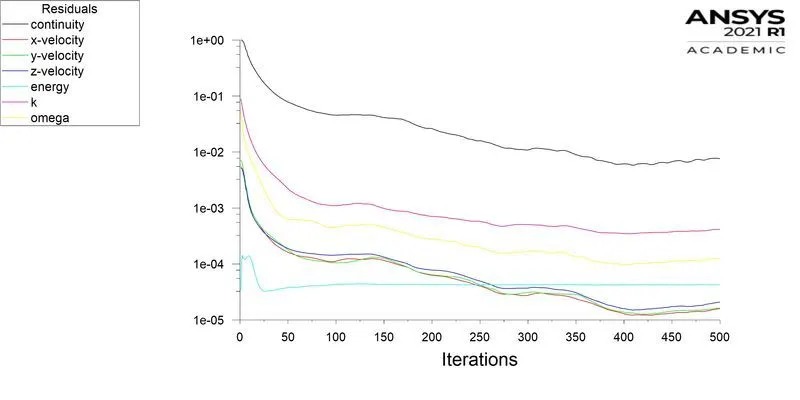
Surface heat transfer coefficient

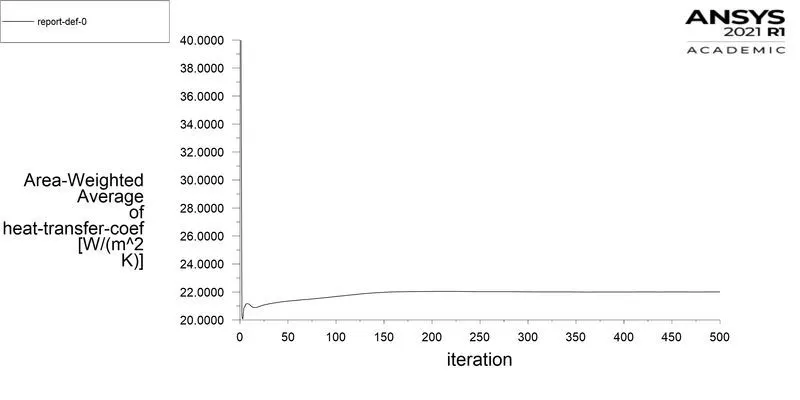
Surface heat transfer coefficient:22.003929w/m^2k

COUPLED METHOD

Residual plot

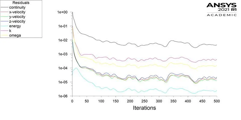
Surface heat transfer coefficient

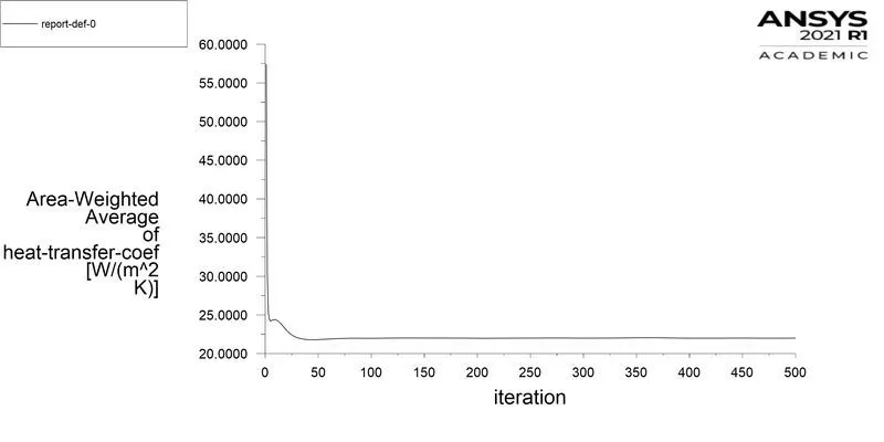
Surface heat transfer coefficient:21.995436w/m^2k

Surface heat transfer coefficient values for three different types of pressure-based solvers

Element size Number of elements Number of nodes HTC(SIMPLE) HTC(SIMPLE) HTC(COUPLED)

0.15M 135747 27104 21.927121W/M^2K 22.003929W/M^2K 21.995436W/M^2K

The above table represents the value of the surface heat transfer coefficient value from the three different pressure-velocity schemes viz SIMPLE, SIMPLEC, COUPLED. The values of heat transfer coefficient is exactly close for SIMPLEC and COUPLED. Both SIMPLE and SIMPLEC are segregated schemes where pressure and velocity coupling are solved sequentially, take less memory, but involves a lot of computational time. The COUPLED scheme, on the other hand, solves pressure and velocity equation instantaneously saves a lot of computational time, and require more memory.

CHT analysis of exhaust port with finer mesh

First refinement

Element size:90mm

Since the value of the heat transfer coefficient takes the value of the first cell near the wall, so it can be inferred that the Y+ value will be in the viscous sub-layer which is taken to be 1.

Steps involved in calculating the first cell height.

Reynolds number = p * v* L/m

=1.225*5*0.17/1.7894e - 05

=58189.8960

The characteristics length is taken as the inlet dia.

Skin friction coefficient,Cf = 0.058/R^0.2e

= 0.00646

Wall shear stress formula,Tw = 0.5 * Cf * P * v^2

=0.5 * 1.225 * 25 * 0.00646

=0.0989 Pa

Frictional velocity formula,Ut = (Tw/p)

=0.2841m/sec

Now,y + = <y * Ut * P/m

since Y + =1

therefore <y = m/Ut * P

=0.000051412m

=0.05141621mm

Inflation

Nunber of inflation layer:6

Growth rate :1.2

Inflation option:First layer thickness

First layer Thickness := 0.05141621mm

Captured curvature is set to yes.

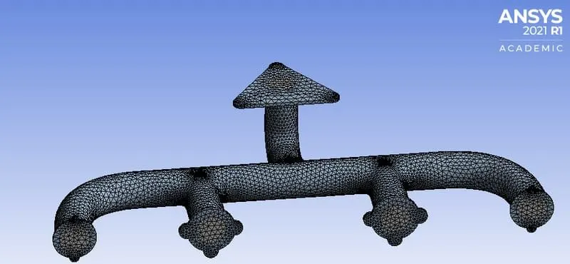
Mesh quality

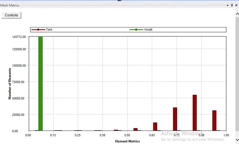
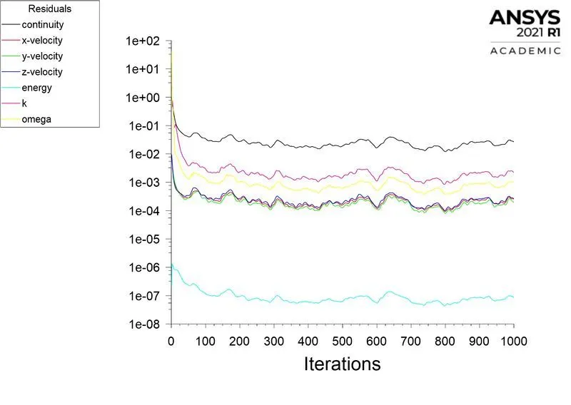
Residual plot

Surface heat transfer coefficient

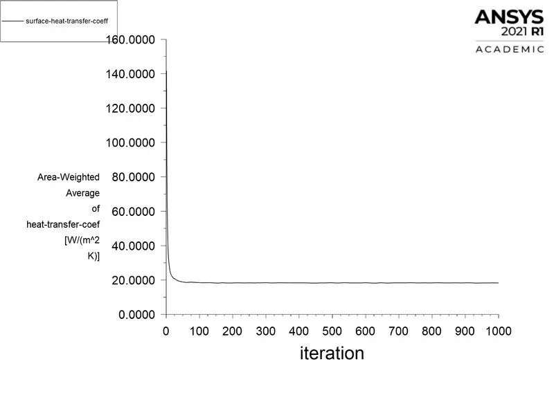
Mesh statistics and surface heat transfer coefficient

Element size 0.09mor90mm

Number of elements 279515

Number of nodes 99980

Y+ 1

First cell height 0.0000514162m or 0.05141621mm

Heat transfer coefficient 18.298713w/m^2k

Second refinement

Element size:80mm

Number of inflation layer:10

First layer thickness:0.05141621mm

Growth rate:1.2

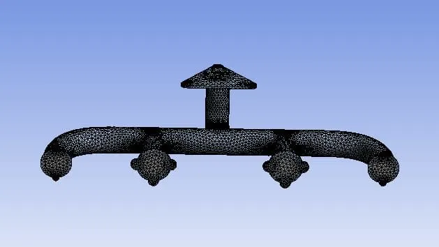
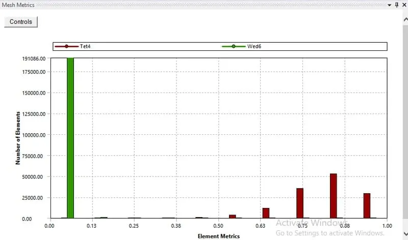
Mesh quality

Residual plot

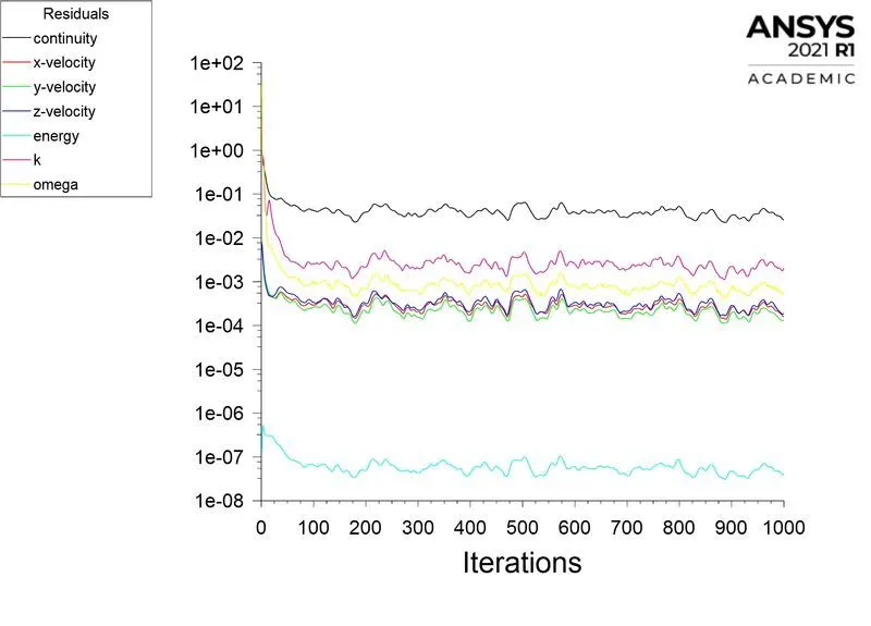
Surface heat transfer coefficient

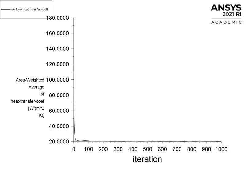
Mesh statistics and surface heat transfer coefficient

Element size 0.08m or 80mm

Number of elements 376380

number of nodes 148719

Y+ 1

First cell Height 0.0000514162m or 0.05141621mm

Heat Transfer coefficient 20.442849w/m^2k

Final refinement

Element size: 70mm

Number of inflation layer:10

First layer thickness : 0.05141621mm

Growth rate :1.2

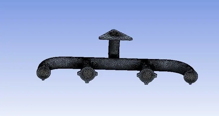
Mesh quality

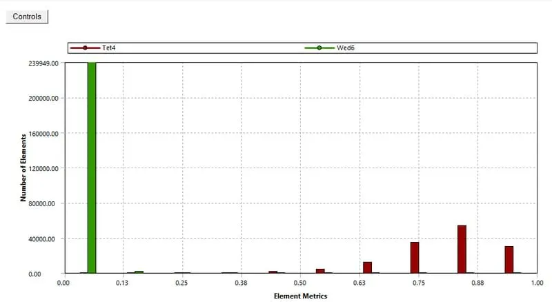
Residual plot

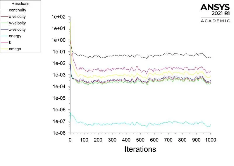
Surface heat transfer coefficient

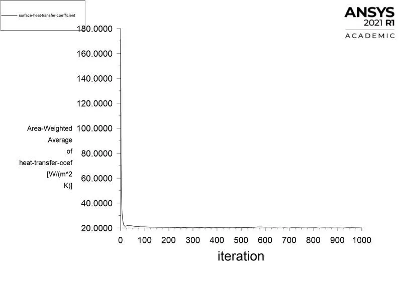
Mesh statistics and surface heat transfer coefficient

Element size 0.07m or 70mm

Number of elements 385926

Number of nodes 151317

Y+ 1

First cell height 0.0000514162m or 0.05141621mm

Heat transfer coeffcient 20.715112w/m^2k

Analytical solution

The reynolds number for the given flow is 58189.8960 which suggests that the flow is turbulent in nature,the Dittus Bolter heat transfer coefficient relation can be used to determine the Nusselt number which is described mathematically as follows

Nud = 0.023 * Re^4/5 D *Pr^n

where pr = m 8 Cp/k

where m is the dynamic viscosity of the fuid in Kg/m-sec = 1.7894e-05kg/m-sec

k is the thermal conductivity of the material in w/mk=0.0242 w/mk

Cp is the specific heat capacity of the Fluid at constant pressure = 1006.43J/kgk

therefore Pr = m *Cp/k = 0.744

n is constant 0.3 heat transfer takes place from fluid to solid.

Therfore convective heat transfer coefficient h = Nu * k/D

19.4287w/m^2k

Comparision of all cases

Element size Number of elements Number of nodes First of cell height Y+ Inflation layer surface heat transfer coefficient Surface heat transfer coefficient Deviation %Deviation

(Numerical value) (Analytical solution)

0.15m 135747 27104 N/A N/A N/A 21.995436w/m^2k 2.566736 13.2

0.09m 279515 99980 6 18.298713w/m^2k 19.4287w/m^2k -1.129987 -5.81

0.08m 376380 148719 0.0000814162m 1 10 20.442849w/m^2k 1.01419 5.21

0.07m 385926 151317 10 20.7151112w/m^2k 1.286412 6.62

Results

The temperature along plane -1 located at the exhaust section of the port.

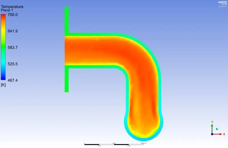
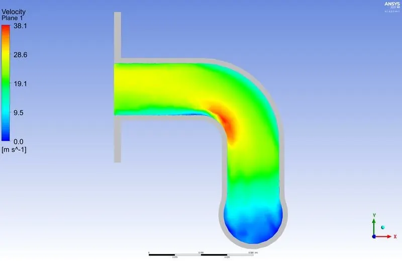
The velocity along plane-1 located at the exhaust section of the port

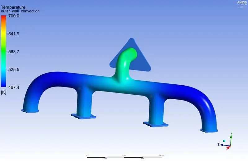
Temperature at outer convection wall.

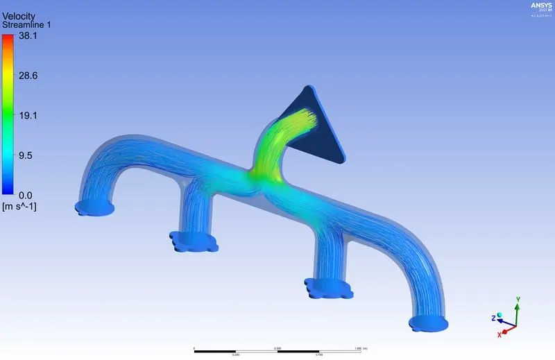
streamline representation of velocity

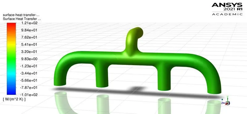
surface heat transfer coefficient

Conclusion

• The CHT analysis on the exhaust port was simulated successfully on ANSYS-FLUENT.
• The pressure-based, coupled scheme solver is used to discretize the whole geometry.
• The analytical value of the heat transfer coefficient is19.4287W/m2K.
• The deviation of numerical heat transfer coefficient values from the analytical solution was found to be within5% to 10%for the second and final mesh refinement are found to be in compliance with the industrial standards.
• The grid independence test was also observed during mesh refinement. The value of the heat transfer coefficient for the second and final mesh refinement are close to each other. It is important that we limit ourselves to the second refinement only to save the computational time and cost of the project.
• The value of the heat transfer coefficient is located in the cell adjacent to the wall which allows us to choose the value of Y+=1 (viscous sublayer) and the turbulent model k−ωSST.
• The presence of the boundary layer is quite visible near the inlet of the pipe where the viscous force makes the velocity near the wall to be zero causing a no-slip condition to occur., but as the flow is turbulent in nature (Reynolds number58189.8960) the velocity profile goes from flat to the flutter and the boundary layer vanishes at the outlet.
• The velocity at the outlet is higher than the velocity at the inlet can be attributed to the presence of four inlets and one outlet.
• The accuracy of the heat transfer coefficient depends on selecting the suitable value of Y+ and turbulence modelk−ωSST model. The heat transfer coefficient values predicted by CFD were validated against the numerical solution depicted the deviation in the range of5%to10%which is in compliance with industrial standards. However, the accuracy of k−ωSST model itself depends on the accuracy of the analytical solution, flow properties, and geometry. The values predicted by the baseline mesh and the refined mesh were close to each other this can be attributed to the fact that the boundary keeps on growing and declining from the inlet to the outlet owing to change in velocity, thus the value is predominant at the outlet section of the exhaust port.