Week 1- Mixing Tee
OBJECTIVE:
For this challenge, we have created two versions of the mixing tee. One of them is longer than the other.
Our job is to set up steady-state simulations to compare the mixing effectiveness when hot inlet temperature is 360C & the Cold inlet is at 190C.
Use the k-epsilon and k-omega SST model for the first case and based on your judgment use the more suitable model for further cases. Giving the reason for choosing a suitable model is compulsory.
1.Case 1
- Short mixing tee with a hot inlet velocity of 3m/s.
- Momentum ratio of 2, 4.
2.Case 2
- Long mixing tee with a hot inlet velocity of 3m/s.
- Momentum ratio of 2, 4.
INTRODUCTION:
The function of mixing Tee is to provide proper mixing of quantities to get the desired result at the outlet.
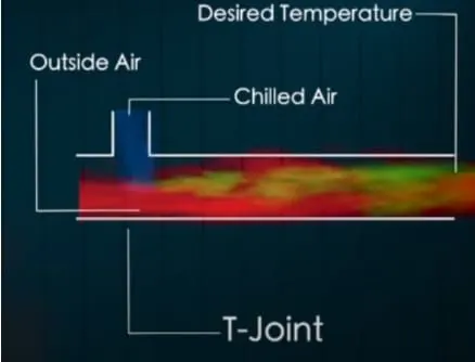
By controlling the velocity of chilled air we can get the desired temperature in the room.
ANSYS WORKFLOW:
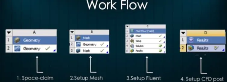
GEOMETRY: Construct a two or three dimensional representation of the object to be modelled and tested using the work plane coordinate system within ANSYS.
MESH: At this point ANSYS understands the makeup of the part. Now define how the modelled system should be broken down into finite pieces.
SETUP: The case setup will be done using ansys fluent
SOLUTION: Ansys fluent where run time result visualization is done
RESULTS: Post processing of results will be done here using CFD-post
SHORT TEE:
GEOMETRY SETUP:
The computational models are uploaded to the Ansys Space Claim as a step file.
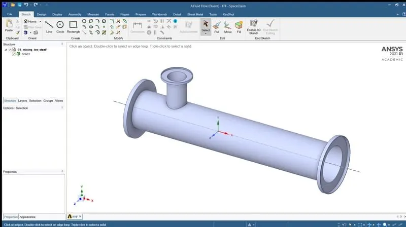
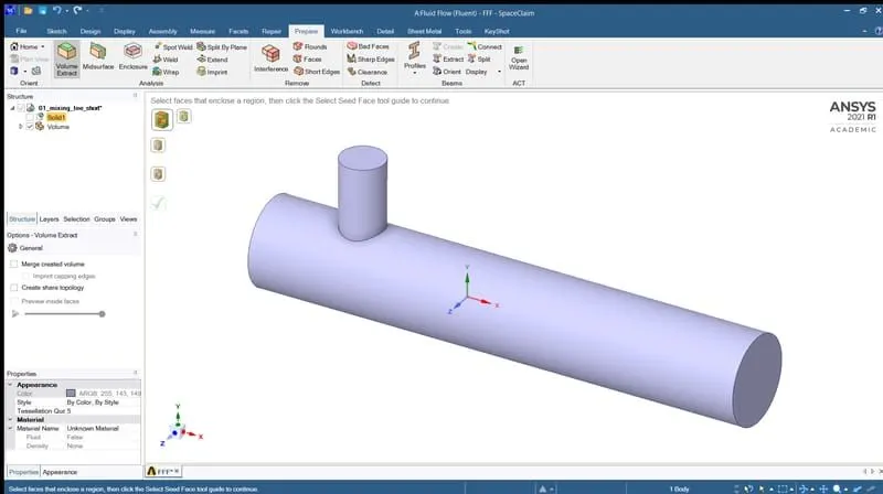
In this project, we are interested in performing fluid flow analysis through the geometry, hence we used the volume extraction option to extract the fluid volume from the geometry. Then the solid model is suppressed for physics from the fluid model to create mesh at the interested region.
MESH GENERATION:
The boundary names inlet_x, inlet_y, outlet and wall are defined using the named selection option.
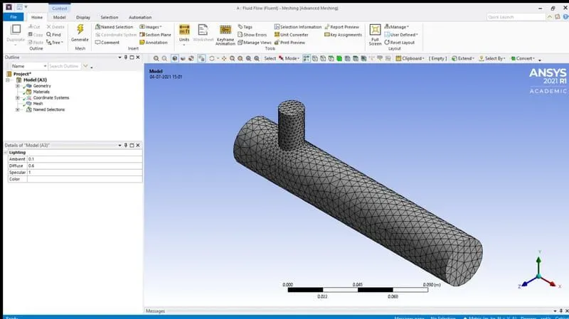
After generating the mesh, the number of nodes and elements are investigated using the statistics option. Then the mesh quality is checked by choosing the mesh metrices option in quality section.
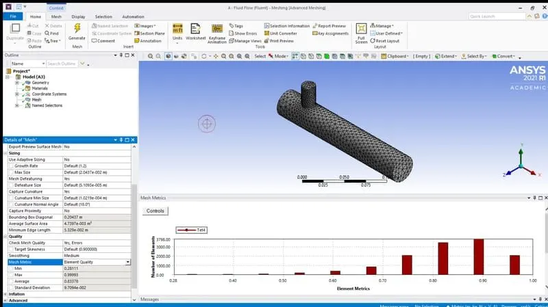
The element quality should not be less than 5%. In our case minimum mesh quality is 30%, so we can move ahead.
SETUP AND SOLUTION:
CASE 1:
- Short mixing Tee with a hot inlet velocity of 3m/s
- Momentum ratio of 2,4
CASE 1.1:
- Short mixing Tee with a hot inlet velocity of 3m/s
- Momentum ratio of 2
SHORT TEE (MR=2 AND HOT INLET VELOCITY = 3m/s)
SETUPS
K-EPSILON K-OMEGA
SOLVER TYPE Pressure based Pressure based
VELOCITY FORMULATION Absolute Absolute
TIME Steady Steady
VISCOUS MODEL Realizable K-epsilon with standard wall function K-omega SST model
MATERIAL Air Air
CELL ZONES Fluid type : air Fluid type : air
· Inlet_x (velocity inlet) · Inlet_x (velocity inlet)
Velocity magnitude 3m/s Velocity magnitude 3m/s
Temperature - 36'c Temperature - 36'c
· Inlet_y (velocity inlet) · Inlet_y (velocity inlet)
Velocity magnitude 6m/s Velocity magnitude 6m/S
BOUNDARIES Temperature – 19'c Temperature – 19'c
· Outlet (pressure outlet)· Outlet (pressure outlet)
Gauge pressure – 0 pa Gauge pressure – 0 pa
· Walls – stationary walls· Walls – stationary walls
The hybrid scheme is used for initialization and the no. of iterations are setup and then click on calculate option.
RESULTS:
K-EPSILON MODEL:
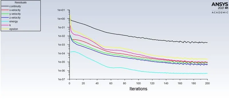
RESIDUAL PLOT:
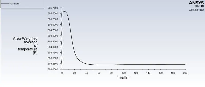
AREA WEIGHTED AVERAGE:
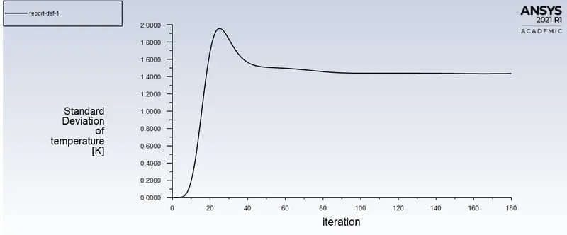
STANDARD DEVIATION:
CONTOUR PLOT:
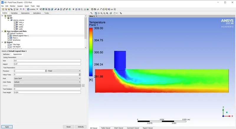
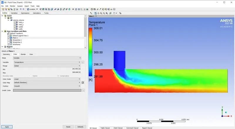
TEMPERATURE CONTOUR:
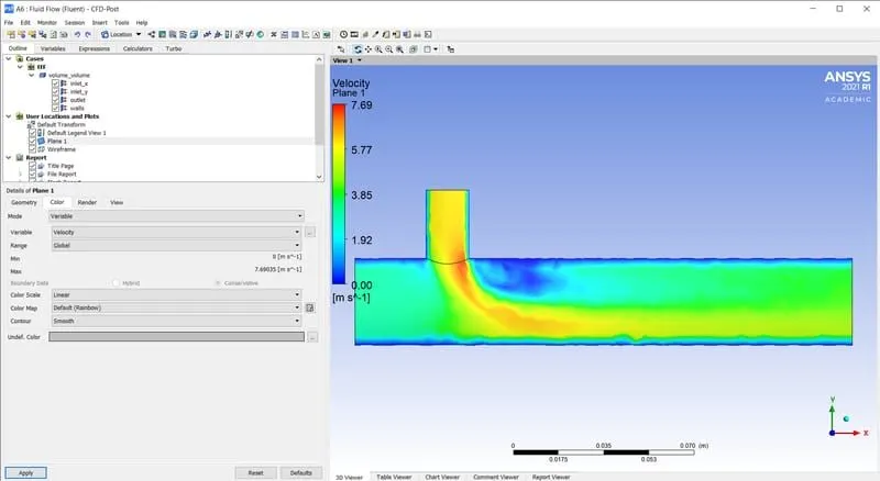
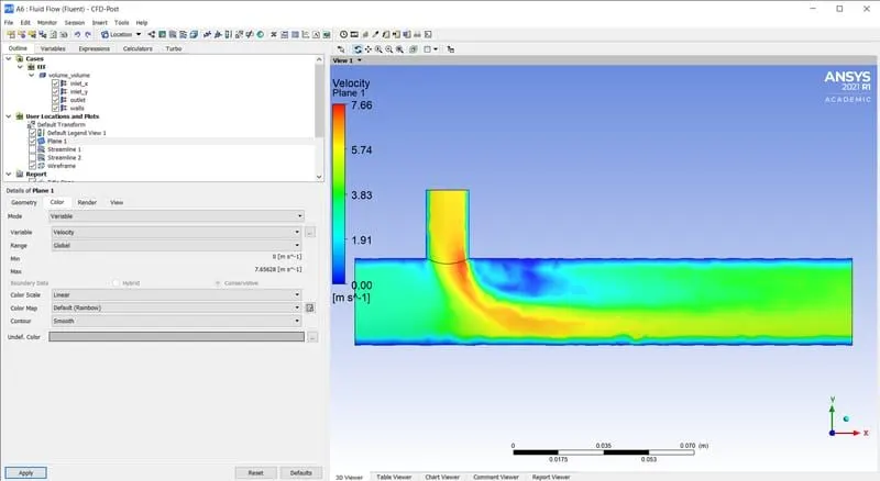
VELOCITY CONTOUR:
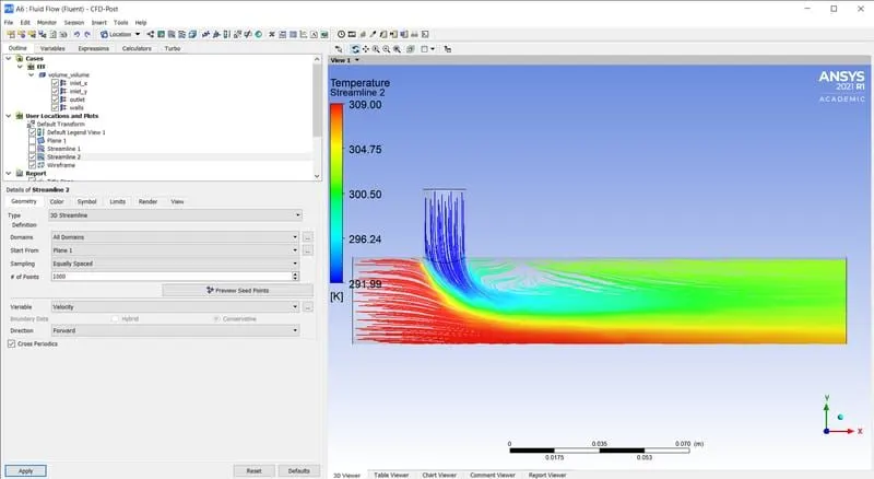
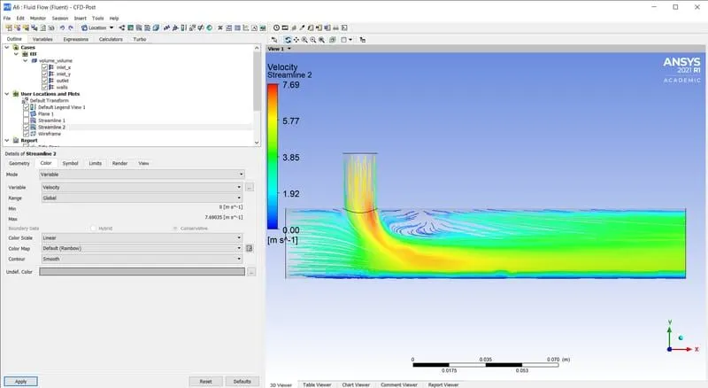
STREAMLINE PLOT:
TEMPERATURE:
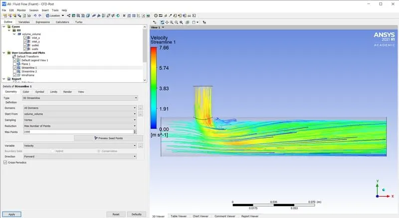
VELOCITY:
K-OMEGA MODEL:
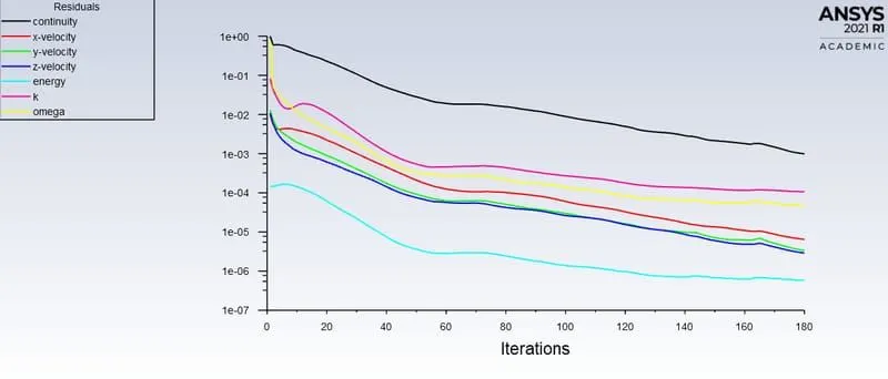
RESIDUAL PLOT:
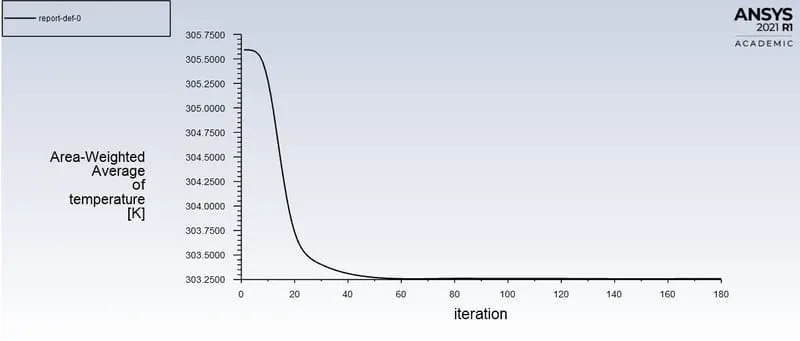
AREA WEIGHTED AVERAGE:
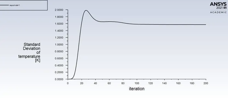
STANDARD DEVIATION:
CONTOUR PLOT:
TEMPERATURE CONTOUR:
VELOCITY CONTOUR:
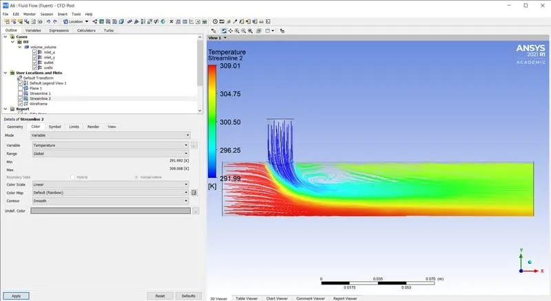
STREAMLINE PLOT:
TEMPERATURE:
VELOCITY:
SUMMARY:
SHORT TEE (MR = 2)
K-EPSILON K-OMEGA
AVERAGE OUTLET TEMPERATURE [K] 303.413 303.458
STANDARD DEVIATION 1.5 1.6
NO OF ITERATIONS 150 170
CASE 1.2:
- Short mixing Tee with a hot inlet velocity of 3m/s
- Momentum ratio of 4
SHORT TEE (MR=2 AND HOT INLET VELOCITY = 3m/s)
SETUPS
K-EPSILON K-OMEGA
SOLVER TYPE Pressure based Pressure based
VELOCITY FORMULATION Absolute Absolute
TIME Steady Steady
VISCOUS MODEL Realizable K-epsilon with standard wall function K-omega SST model
MATERIAL Air Air
CELL ZONES Fluid type : air Fluid type : air
· Inlet_x (velocity inlet) · Inlet_x (velocity inlet)
Velocity magnitude 3m/s Velocity magnitude 3m/s
Temperature - 36'c Temperature - 36'c
· Inlet_y (velocity inlet) · Inlet_y (velocity inlet)
BOUNDARIES Velocity magnitude 12m/s Velocity magnitude 12m/s
Temperature – 190c Temperature – 190c
· Outlet (pressure outlet) · Outlet (pressure outlet)
Gauge pressure – 0 pa Gauge pressure – 0 pa
· Walls – stationary walls · Walls – stationary walls
The hybrid scheme is used for initialization and the no. of iterations are setup and then click on calculate option.
RESULTS:
K-EPSILON MODEL:
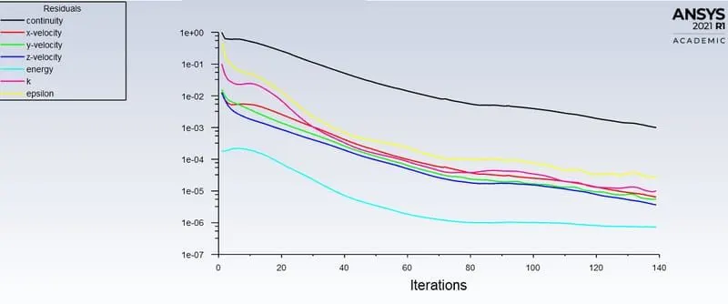
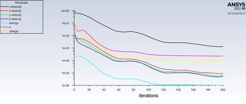
RESIDUAL PLOT:
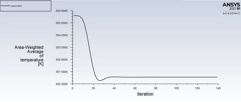
AREA WEIGHTED AVERAGE:
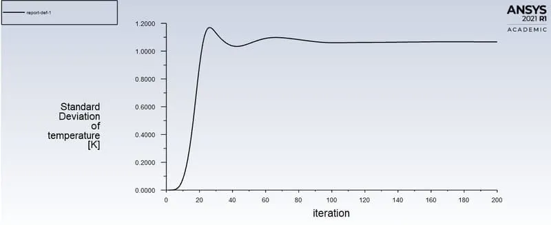
STANDARD DEVIATION:
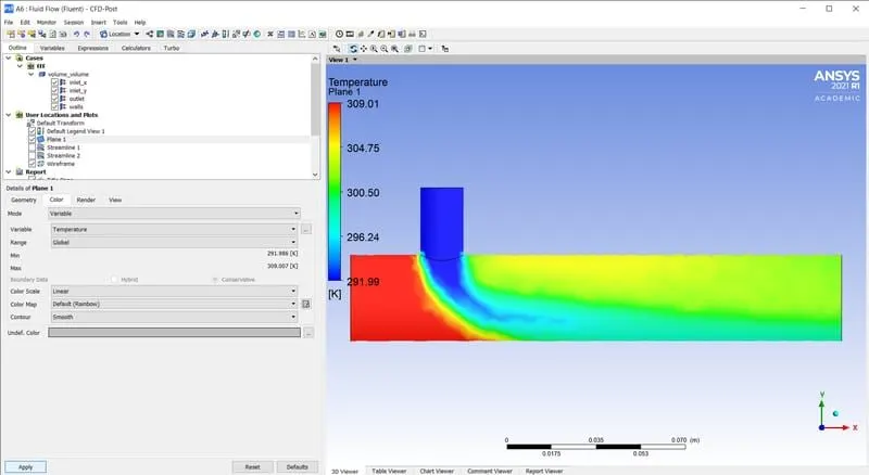
CONTOUR PLOT:
TEMPERATURE CONTOUR:
VELOCITY CONTOUR:
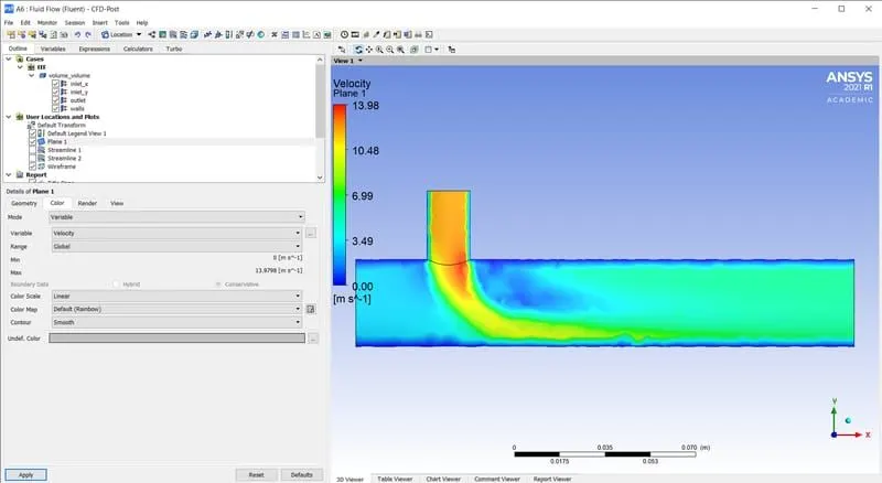
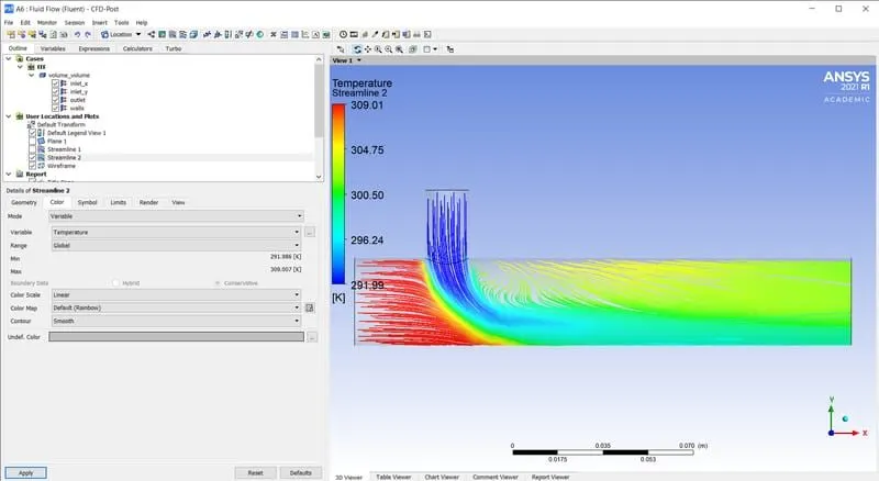
STREAMLINE PLOT:
TEMPERATURE:
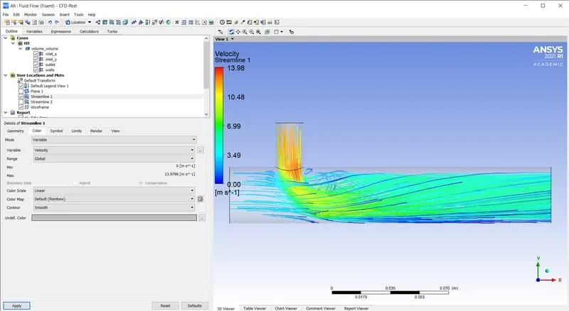
VELOCITY:
K-OMEGA MODEL:
RESIDUAL PLOT:
AREA WEIGHTED AVERAGE:
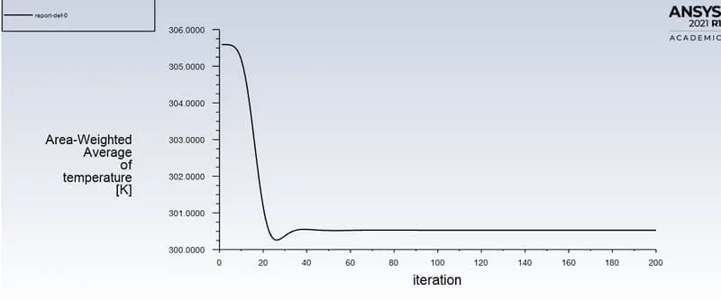
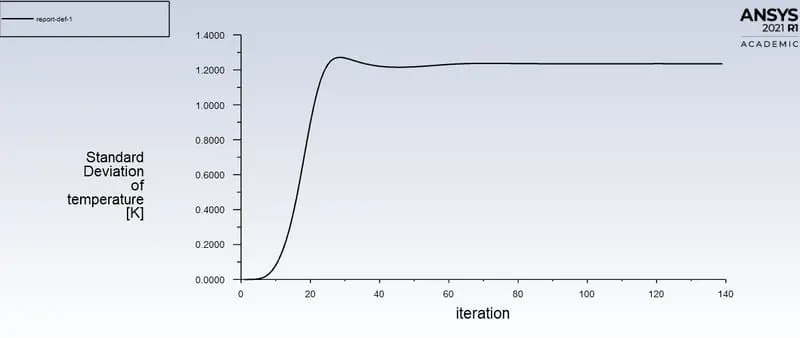
STANDARD DEVIATION:
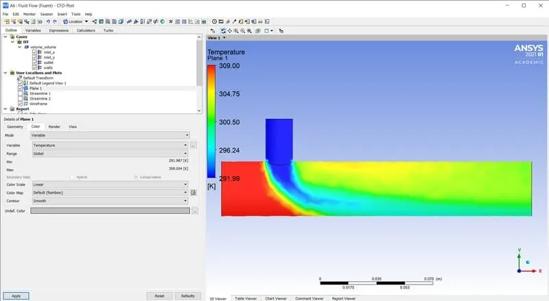
CONTOUR PLOT:
TEMPERATURE CONTOUR:
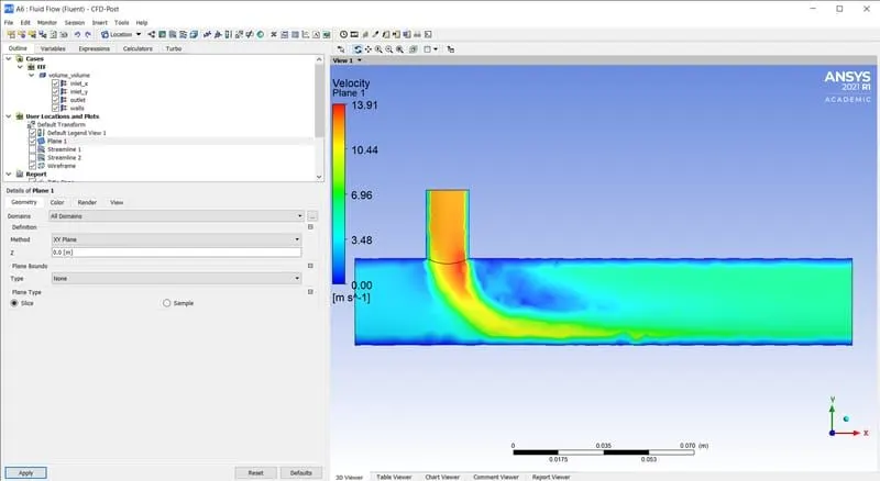
VELOCITY CONTOUR:
STREAMLINE PLOT:
TEMPERATURE:
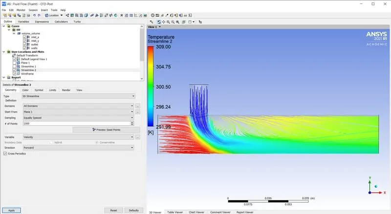
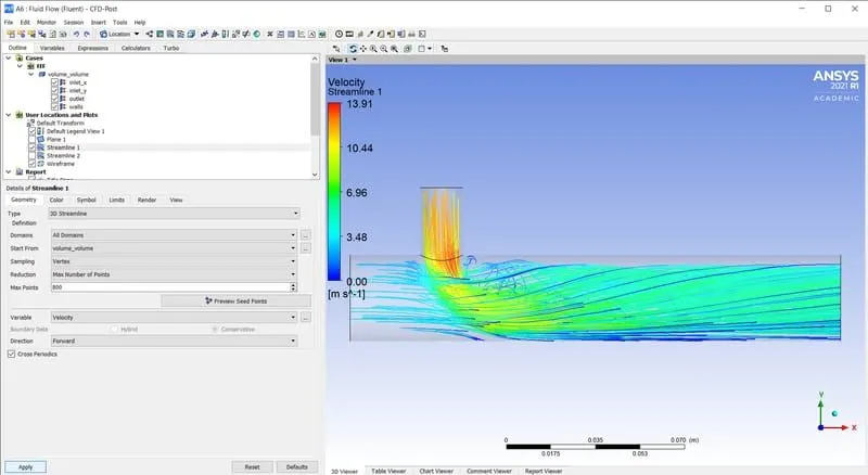
VELOCITY:
SUMMARY:
SHORT TEE (MR = 4)
K-EPSILON K-OMEGA
AVERAGE OUTLET TEMPERATURE [K] 300.396 300.38
STANDARD DEVIATION 1.1 1.2
NO OF ITERATIONS 130 160
ANALYTICAL SOLUTION:
MOMENTUM RATIO 2:
- Mass of hot fluid (mh) = rho*a*Vh = 997*0.0009*3 = 2.69 kg/s
- Mass of cold fluid (mc) = rho*a*Vc = 997*0.0009*6 = 1.35 kg/s
- Temperature of mixture (Tmixture) = (mh*Th + mc*Tc)/(mc + mh) = 30.3190c = 303.319k
MOMENTUM RATIO 4:
- Mass of hot fluid (mh) = rho*a*Vh = 997*0.0009*3 = 2.69 kg/s
- Mass of cold fluid (mc) = rho*a*Vc = 997*0.0009*12 = 2.3928 kg/s
- Temperature of mixture (Tmixture) = (mh*Th + mc*Tc)/(mc + mh) = 27.990c = 300.99k
CONCLUSION:
AVERAGE OUTLET TEMPERATURE:
On comparing the both models with analytical solution we got nearly the same results.
ITERATIONS TO CONVERGE:
No. of iterations taken to converge is less for Realisable K-epsilon model than K-omega SST model.
STANDARD DEVIATION:
The standard deviation of k-epsilon model is less than k-omega model which shows the better mixing efficiency in k-epsilon model.
So based on the above observations the K-epsilon turbulence model is predicting the results accurately in less no. of iterations. So we can use realisable k-epsilon model for case 2
LONG TEE:
GEOMETRY SETUP:
The computational models are uploaded to the Ansys Space Claim as a step file.
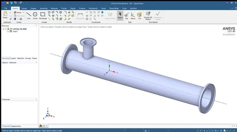
In this project, we are interested in performing fluid flow analysis through the geometry, hence we used the volume extraction option to extract the fluid volume from the geometry. Then the solid model is suppressed for physics from the fluid model to create mesh at the interested region.
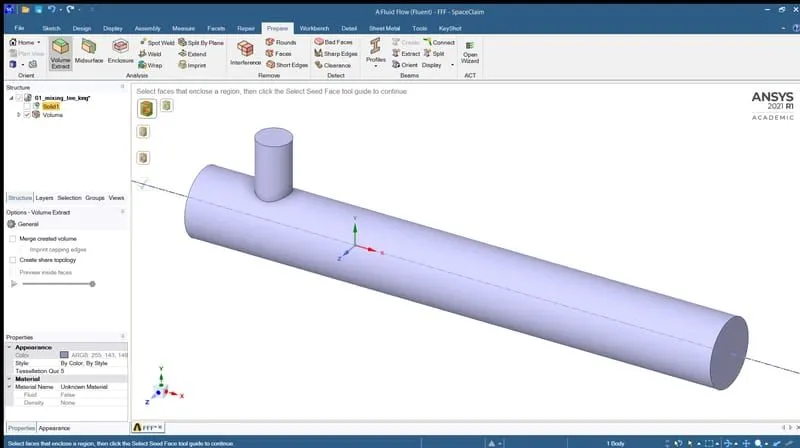
MESH GENERATION:
The boundary names inlet_x, inlet_y, outlet and wall are defined using the named selection option.
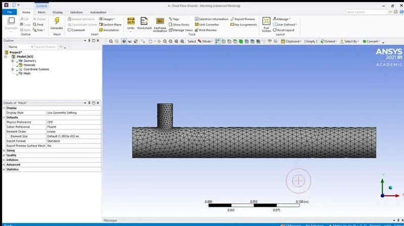
After generating the mesh, the number of nodes and elements are investigated using the statistics option. Then the mesh quality is checked by choosing the mesh metrices option in quality section.
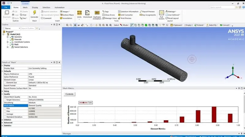
The element quality should not be less than 5%. In our case minimum mesh quality is 30%, so we can move ahead.
SETUP AND SOLUTION:
CASE 2:
- Long mixing tee with a hot inlet velocity of 3m/s.
- Momentum ratio of 2, 4.
CASE 2.1:
- Long mixing tee with a hot inlet velocity of 3m/s.
- Momentum ratio of 2.
LONG TEE (MR=2 AND HOT INLET VELOCITY 3m/s)
SETUPS
K-EPSILON
SOLVER TYPE Pressure based
VELOCITY FORMULATION Absolute
TIME Steady
VISCOUS MODEL Realizable K-epsilon with standard wall function
MATERIAL Air
CELL ZONES Fluid type : air
· Inlet_x (velocity inlet)
Velocity magnitude 3m/s
Temperature - 360c
· Inlet_y (velocity inlet)
Velocity magnitude 6m/s
BOUNDARIES Temperature – 190c
· Outlet (pressure outlet)
Gauge pressure – 0 pa
· Walls – stationary walls
The hybrid scheme is used for initialization and the no. of iterations are setup and then click on calculate option.
RESULTS:
RESIDUAL PLOT:
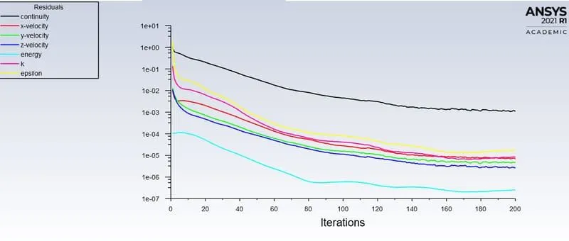
AREA WEIGHTED AVERAGE:
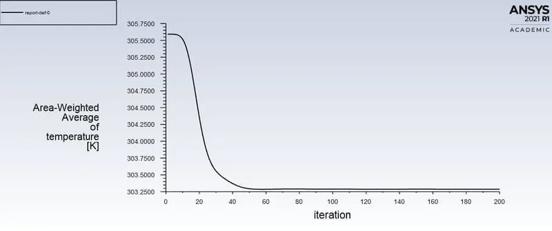
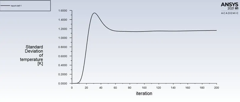
STANDARD DEVIATION:
CONTOUR PLOT:
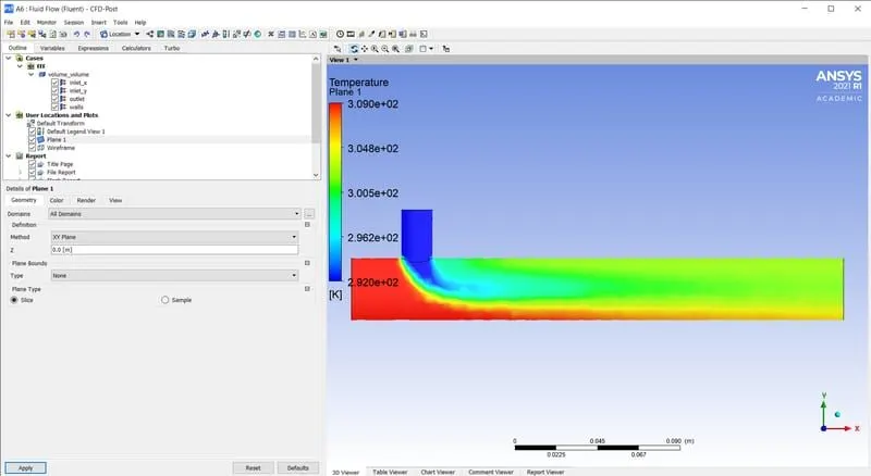
TEMPERATURE CONTOUR:
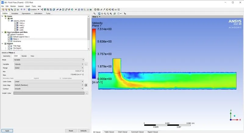
VELOCITY CONTOUR:
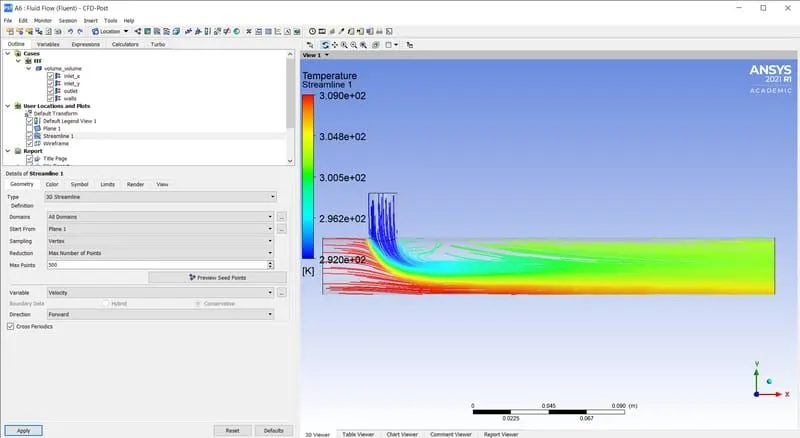
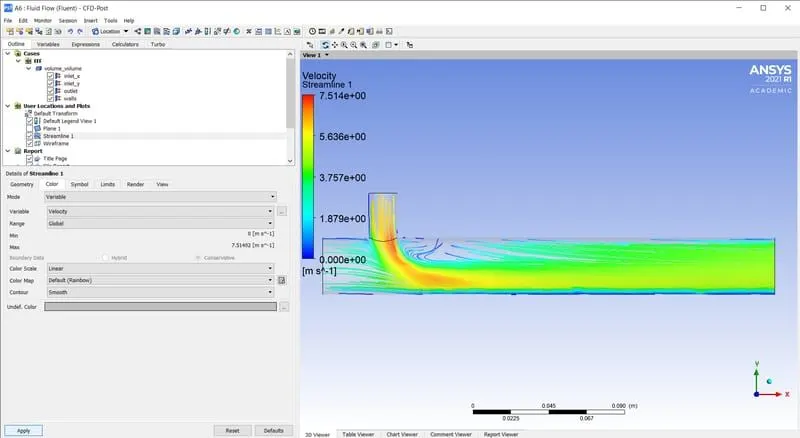
STREAMLINE PLOT:
TEMPERATURE:
VELOCITY:
CASE 2.2:
- Long mixing tee with a hot inlet velocity of 3m/s.
- Momentum ratio of 4.
LONG TEE (MR=2 AND HOT INLET VELOCITY 3m/s)
SETUPS
K-EPSILON
SOLVER TYPE Pressure based
VELOCITY FORMULATION Absolute
TIME Steady
VISCOUS MODEL Realizable K-epsilon with standard wall function
MATERIAL Air
CELL ZONES Fluid type : air
BOUNDARIES · Inlet_x (velocity inlet)
Velocity magnitude 3m/s
Temperature - 360c
· Inlet_y (velocity inlet)
Velocity magnitude 12m/s
Temperature – 190c
· Outlet (pressure outlet)
Gauge pressure – 0 pa
· Walls – stationary walls
The hybrid scheme is used for initialization and the no. of iterations are setup and then click on calculate option.
RESULTS:
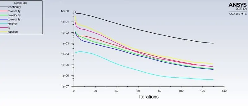
RESIDUAL PLOT:
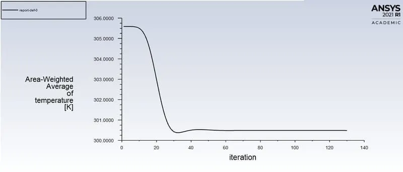
AREA WEIGHTED AVERAGE:
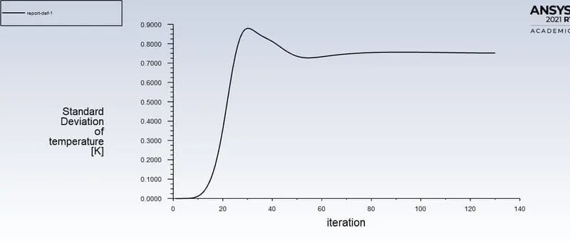
STANDARD DEVIATION:
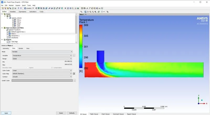
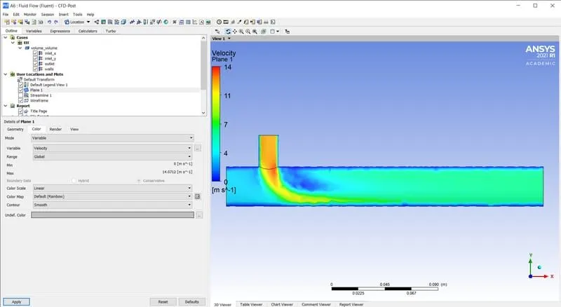
CONTOUR PLOT:
TEMPERATURE CONTOUR:
VELOCITY CONTOUR:
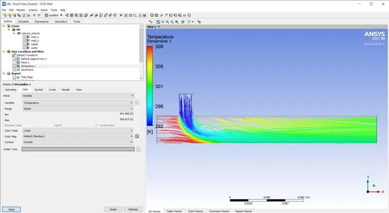
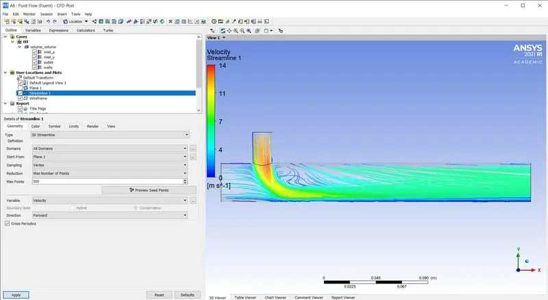
STREAMLINE PLOT:
TEMPERATURE:
VELOCITY:
SUMMARY:
LONG TEE (MR = 2) LONG TEE (MR = 4)
AVERAGE OUTLET TEMPERATURE [K] 303.367 300.449
STANDARD DEVIATION 1.2 0.8
NO OF ITERATIONS 180 130
COMPARISON OF BOTH LONG AND SHORT TEE:
K-EPSILON REALIZABLE MODEL
GEOMETRY MOMENTUM RATIO CELL COUNT AVERAGE OUTLET TEMPERATURE [K] NO. OF ITERATIONS STANDARD DEVIATION
SHORT TEE 2 12583 303.413 150 1.5
SHORT TEE 4 12583 300.396 130 1.1
LONG TEE 2 15368 303.367 180 1.2
LONG TEE 4 15368 300.449 130 0.8
OVERALL DISCUSSION:
AVERAGE OUTLET TEMPERATURE:
Irrespective of length of the mixing Tee, the average outlet temperature on both cases are quite same.
MOMENTUM RATIO:
- As momentum ratio increases, the velocity of cold inlet fluid increases and due to high relative velocity between the fluid it experiences higher turbulence and therefore the outlet fluid temperature decreases.
- For momentum ratio 2, the average outlet fluid temperature is 303k whereas for momentum ratio 4 the average outlet fluid temperature is 300k. From these we can say that there will be a drop in temperature if momentum ratio increases.
- In order to obtain better mixing the velocity of cold air is important. By increasing the cold fluid velocity the outlet temperature gets reduced.
NO. OF ITERATIONS:
The longer Tee takes more time to converge than short Tee.
CONCLUSION:
- Higher the momentum ratio, higher will be the mixing efficiency of Tee joint.
- Increasing the length of the pipe doesn’t serve the purpose of mixing efficiently. So, it is efficient to use short pipe.
GRID INDEPENDENCY TEST:
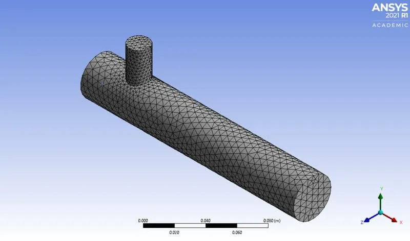
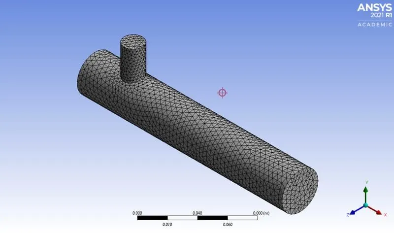
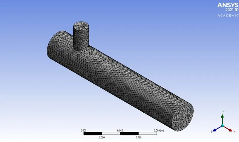
Short Tee model is selected for grid dependence test.
MESH GENERATION:
5mm:
4mm:
3mm:
RESULTS:
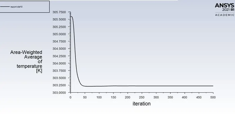
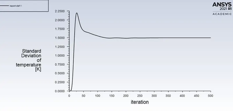
5mm:
RESIDUAL PLOT:
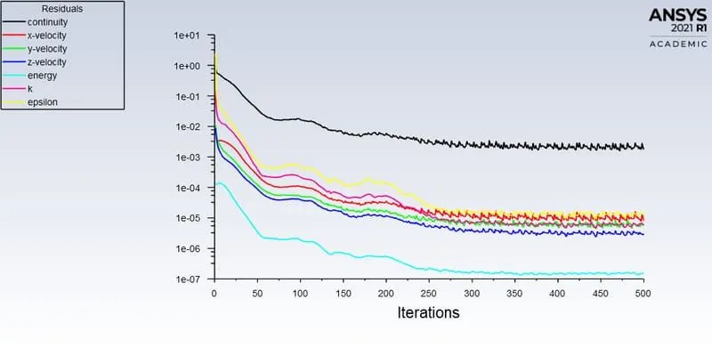
AREA WEIGHTED AVERAGE OF TEMPERATURE:
STANDARD DEVIATION OF TEMPERATURE:
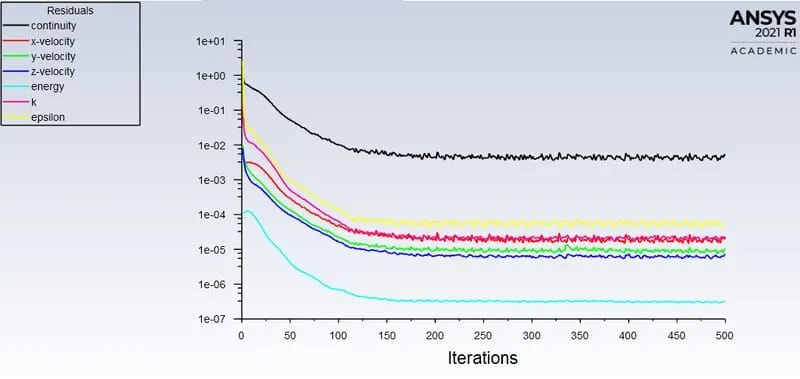
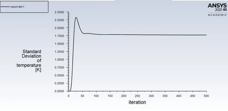
4mm:
RESIDUAL PLOT
STANDARD DEVIATION OF TEMPERATURE:
AREA WEIGHTED AVERAGE OF TEMPERATURE:
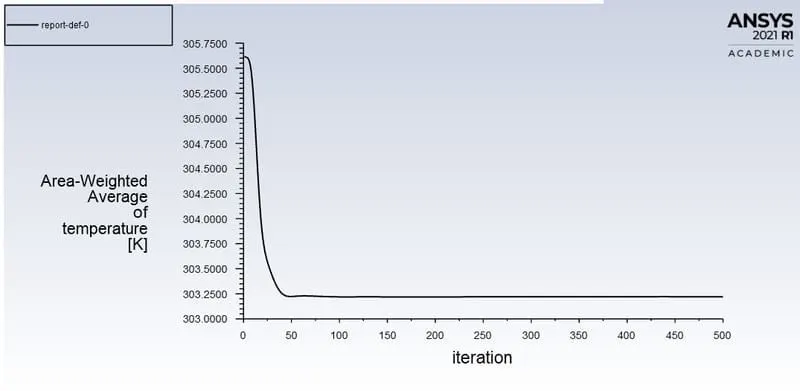
3mm:
RESIDUAL PLOT:
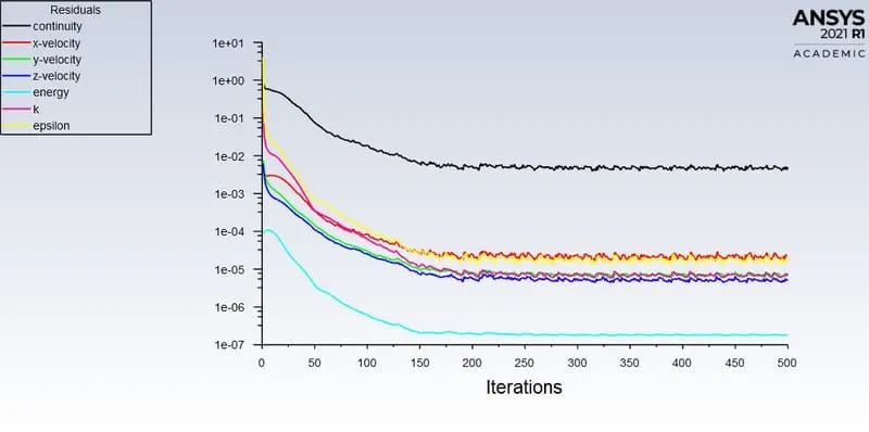
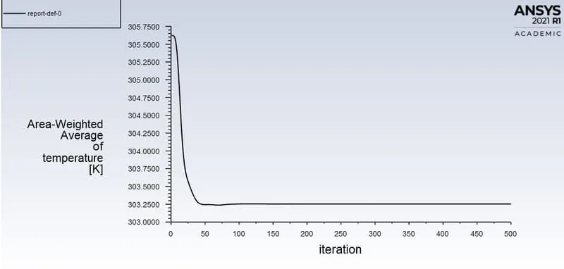
AREA WEIGHTED AVERAGE OF TEMPERATURE:
STANDARD DEVIATION OF TEMPERATURE:
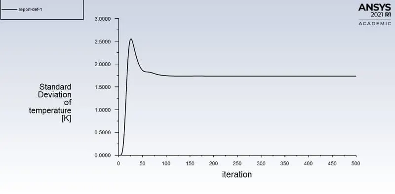
SUMMARY:
MESH SIZE NO. OF ELEMENTS NO. OF NODES AVERAGE OUTLET TEMPERATURE NO. OF ITERATIONS
5mm 16143 3460 303.251 250
4mm 23007 4925 303.246 175
3mm 39921 8369 303.292 210
CONCLUSION:
- The mesh size of 3mm gives the best predicted results than other two mesh size
- Decreasing the mesh size, the average outlet temperature starts approaching towards the analytical results.