Week 3 - Solving second order ODEs
Solving second-order ODEs
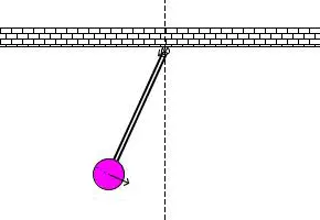
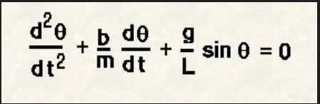
Aim: Write a program to solve the 2nd order ODE equation using Matlab. This ODE represents the equation of motion of a simple pendulum with damping.
What is a Second Order Differential Equation?
A differential equation is an equation that consists of a function and its derivative. A differential equation that consists of a function and its second-order derivative is called a second-order differential equation. Mathematically, it is written as y'' + p(x)y' + q(x)y = f(x), which is a non-homogeneous second order differential equation if f(x) is not equal to the zero function and p(x), q(x) are functions of x. It can also be written as F(x, y, y', y'') = 0. Further, let us explore the definitions of the different types of the second-order differential equation.
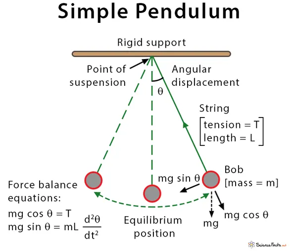
Simple pendulum
The simple pendulum is another mechanical system that moves in an oscillatory motion. It consists of a point mass ‘m’ suspended by means of light inextensible string of length L from fixed support as shown in Fig. 2.8. The motion occurs in a vertical plane and is driven by a gravitational force. The forces which are acting on the mass are shown in the figure. The tangential component of the gravitational force, mg sin θ, always acts towards the mean position θ = 0 opposite to the displacement, restoring force acting tangent to the arc.
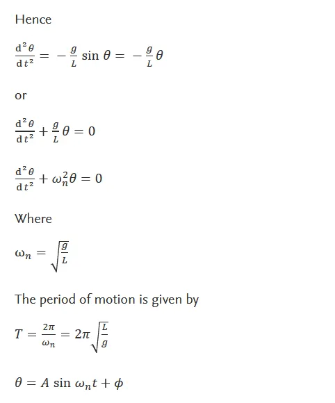
For small displacement sin θ ≅ θ and the motion of the bob is along the arc
1. Inputs required to solve 2nd order ODE equation
  b=0.05;           %Damping Coefficient
  g=9.81;           %Gravity in m/s2,
  l=1;              %Length of the pendulum in m,
  m=0.1;           %Mass of the ball in kg,
Where,
g →gravity in m/s2,
L →length of the pendulum in m,
m →mass of the ball in kg,
b →damping coefficient
2. The single array variable to store the angular displacement & angular velocity is defined as shown. The former is kept as 0.
% initial single array variable condition
  theta=[0;5];
3. Now we need the time limits. This can be provided as a vector of 2 values, the initial and final time, or with a spacing using the linspace function.
% time limits provided as a vector of 2 values, the initial and final time
  t_span=linspace(0,20,300);
Then define an objective function,(i.e. ode_func()). Here we will define the converted 2nd order pendulum ODEs. They are the eqn1 and eqn3 in the CALCULATION. This objective function intakes as, the current time (t), (theta) would be the value of the function at the previous time step and other arguments such as b,g, L, M. The code is as shown:-
% Creating Function for 2nd Order ODE

function [dtheta_dt] = Ode_func(t,theta,b,g,l,m)

  theta1 = theta(1)
  theta2 = theta(2)
  dtheta1_dt = theta2;
  dtheta2_dt = -(b/m)*theta2 -(g/l)*sin(theta1);
  dtheta_dt = [dtheta1_dt; dtheta2_dt];

end
% solving the ODE with formula
[t,results]=ode45(@(t,theta) Ode_func(t,theta,b,g,l,m),t_span,theta);% Plotting
plot(t,results(:,1))
hold on
plot(t,results(:,2))
title('2nd Order ODE')
legend('Angular Displacement','Angular Velocity')
xlabel('Time')
ylabel('Displacement')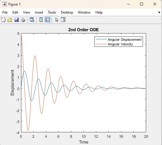
% Crating Animation of Pendulum

for i=1:length(results(:,1))

    x0=0;
    y0=0;

    x1=l*sin(results(i,1));
    y1=-l*cos(results(i,1));

    plot([0.5,-0.5],[0,0],'linewidth',3,'color','GREEN');
    hold on
    plot([x0 x1],[y0 y1],'linewidth',2,'color','BLACK');
    plot(x1,y1,'O','MarkerSize',15,'markerfacecolor','RED');

    grid on
    axis([-2 2 -1.5 1])
    pause(0.003)
    hold off
    M(i) = getframe(gcf);

endfor iterating the position of pendulum at each time framey0=0;
% x and y coordinate of the pivoted end of the pendulumy1=-l*cos(results(i,1));
% x and y coordinate of the non-pivoted end% plots the pivotting line to which the pendulum is oscillating% plots the pendulum co ordinate and length% plots the mass with markersize
% CREATING THE MOVIE

movie(M)
videofile = VideoWriter('Pendulem_Animation.avi','uncompressed AVI')
open(videofile)
writeVideo(videofile,M)
close(videofile) - Thus the Matlab program to solve the 2nd order ODE is successfully completed and the output is verified.
- The plot between angular displacement & time is successfully carried out.
- The plot between angular velocity & time is successfully carried out.
- The animation of pendulum oscillation is successfully carried out.