Week 3 - Solving second order ODEs
Aim:- To solve an ordinary differential equation(ODE) and use calculated information to simulate motion of pendulum.
Objectives:-
1. To solve an ordinary differential equation.
2. Generate a video which simulates the motion of pendulum.
Introduction:-
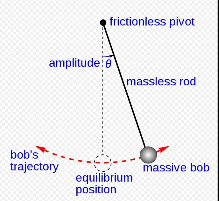
A pendulum is weight suspended from pivot so that it can swing freely. When pendulum is displaced sideways from its resting, it is subjected to restoring force due to gravity that will accelerate it back towords the equilibrium position. When released, the restoring force acting on the pendulum's mass cause it to ocsillate about the equlibrium position, swinging back and forth.
Pendulum have many application and where utilized often before the digital age. They are used in clocks, metronums due to the regularity of their period, in wrecking balls and playground swings, due to their simple way of building up and keeping energy. A simple pendulum consist of a point mass suspended on string or wire that has negligble mass . If the pendulum weight or bob pulled to a relatively small angle from the vertical angle and let it go it will swing back and forth at regular period of frequency.
Ordinary Differential equation:-
An ordinary differential equation, is an equation consist of one or more functions of one independent variable and derivatives of those functions.
Following are ODE equations,
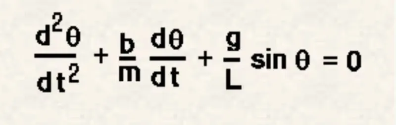
where,
b=Damping Coefficient.
m=Mass of ball.
g=Gravitational Acceleration.
l=Length of pendulum.
Governing Equation:-
`theta = theta1`
`(d theta)/dt = (d theta1)/dt = theta2 ...........(1)`
`(d^2 theta)/dt^2 = (d^2theta1)/dt^2 = d/dt((d theta1)/dt)`
`(d^2 theta)/dt = (d theta2)/dt ...........(2)`
Substituting values from equation (1) and (2) in above equation.
`(d theta2)/dt+ b/m(theta2)+g/m*sin (theta1) = 0`
so,`(d theta1)/dt = theta2`and `(d theta2)/dt=-b/m* theta2 -g/l*sin(theta1)`
Hence `d/dt[theta1,theta2]`is solution vector.
Code Explanation:-
Function Code:- Function is group of statement that together perform a task. In matlab fuctions are defined in seperate file. The name of the file and of function should be same.
% A function program will be called to solve ordinary differential equation of simple pendulum.
function [dtheta_dt] = ode_func(t,theta,b,g,l,m)
theta1 = theta(1)
theta2 = theta(2)
dtheta1_dt = theta2;
dtheta2_dt = -(b/m)*theta2-(g/l)*sin(theta1);
dtheta_dt=[dtheta1_dt;dtheta2_dt];
end
Main code:-
Step1- Start with clear all, close all, clc.
Step2- Assign Input variables such as damping coeff, gravitational acc, length of pendulum and mass of pendulum.
Step3- Define initial condition such as angular displacement, initial velocity and time span.
Step4- To solve ode using ode45 solver.
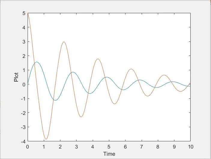
Step5-After calculating variables plot the results. There are two graphs need plot first is anguar displacement Vs time and second one angular velocity with respect to time.
Step6- Create a movieclip using movie command. This file formate is of .avi.
%Main code.
clear all
close all
clc
%Inputs
b=0.05; %............Damping Coeff.
g=9.81; %............Gravitational Acc
l=1; %............Length of pendulum
m=0.1; %...........Mass of Pendulum ball
%Initial Condition
theta_0=[0;5];
%Time Plot
t_span= linspace(0,10,500);
%To solve ODE
[t, result] = ode45(@(t,theta) ode_func(t,theta,b,g,l,m),t_span,theta_0); %..........Eqn to solve ODE
plot(t,result(:,1))
hold on
plot(t,result(:,2))
xlabel("Time')
ylabel('Plot')
&Plotting Results
ct=1;
for i= 1:length (result(:,1))
x_start =0;
y_start=0;
x_end = l*sin(result(i,1));
y_end = -l*cos(result(i,1));
figure(2)
plot([-1,1],[0,0],'linewidth',5);
hold on
plot([x_start x_end],[y_start y_end],'linewidth',3)
hold on
plot(x_end y_end,'o','markersize',20,'markerfacecolor','r')
axis([-1.5 1.5 -1.5 1])
hold off
M(ct)=getframe(gcf)
ct=ct+1
end
movie(M)
Videofile=VideofileWriter('Pendulum Animation.avi','Uncompressed AVI',)
open(Videofile)
writeVideo(Videofile,M)
Close(Videofile)
Results:-
Animation of Simple Pendulum:-