Project 2 - Rankine cycle Simulator
Title :- Rankine Cycle Simulator.
Aim :- Create a Rankine cycle Simulator from a data given in standard thermodynamic library of steam table.
Objectives :-
1. To create a Rankine cycle simulator.
2. To calculate state point of Rankine Cycle.
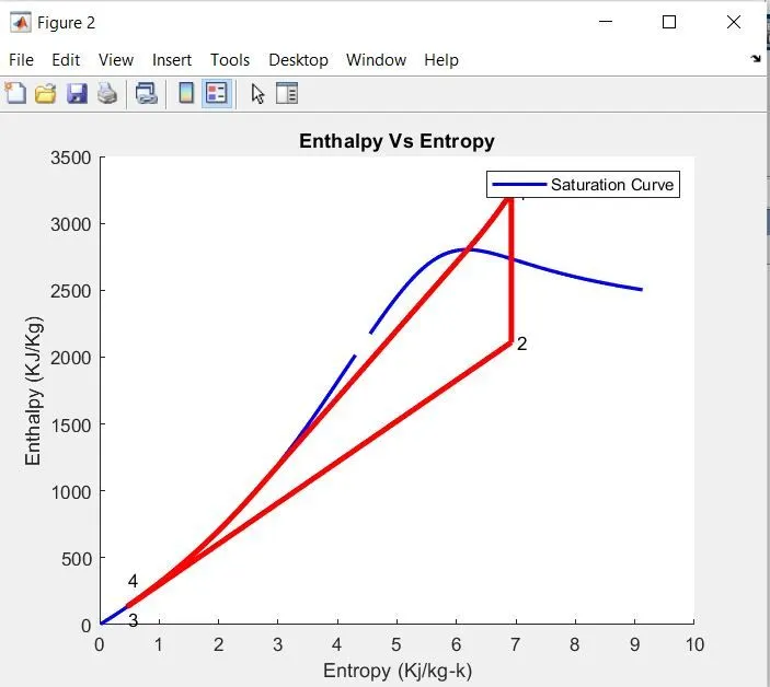
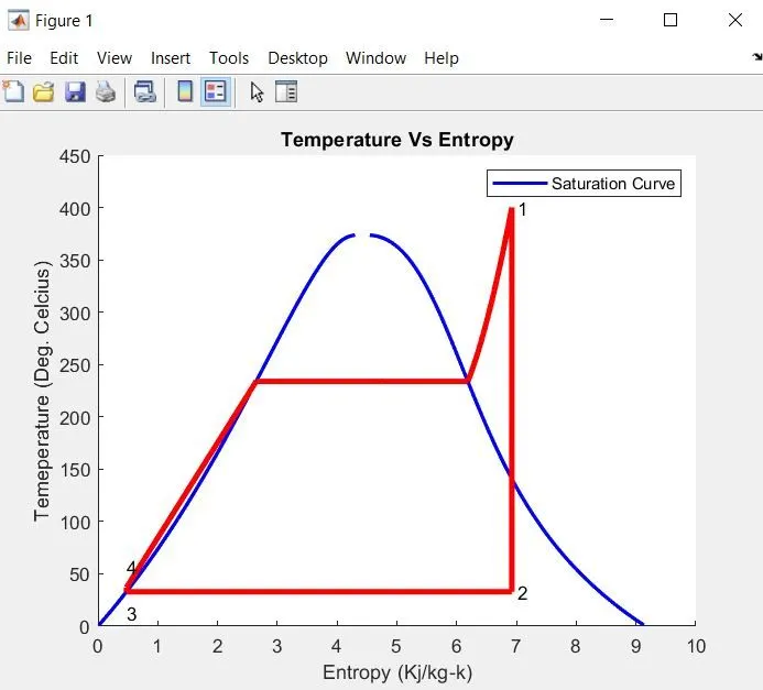
3.To plot the T-S and H-S curve for given input in Rankine Cycle.
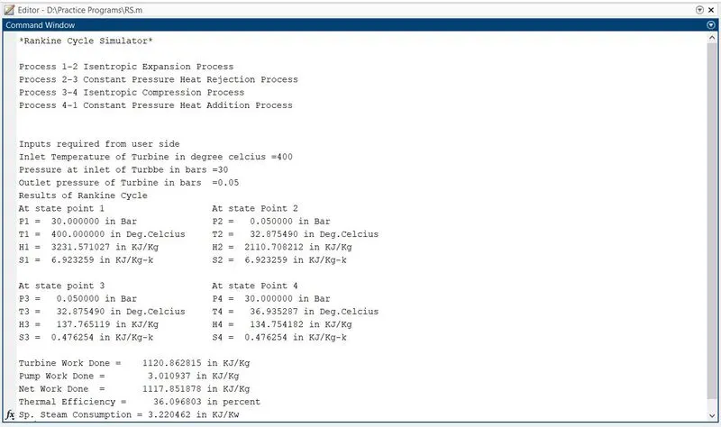
4. To get output in the command window for each state point in cycle.
Theory :-
Rankine Cycle
Rankine cycle closely describes the process by which steam engine commonly found in thermal power generation plant harness the thermal energy of the fuel or other heat source to generate the electricity. Possible heat sources includes combustion of fossil fuels such as coal, natural gas or oil. Common heat sinks include ambient air above or around a facility and bodies of water such as rivers, ponds, and oceans.
The ability of a Rankine engine to harness energy depends on the relative temperature difference between the heat source and heat sink. The greater the differential, the more mechanical power can be efficiently extracted out of heat energy, as per carnot therom. The efficiency of rankine cycle is limited by high heat of vapourization of workinf fluid. Unless the temperature reaches the super critical level in the boiler. The temperature range over an cycle operate is small.
Rankine cycle generally used in closed loop were the working fluid is reused. The water vapour with condensed droplets often seen billowing from powerstation is created by the cooling system. This 'exhaust' heat is represented by the "Qout" flowing out of the lower side of the cycle shown in the T–s diagram below. Cooling towers operate as large heat exchangers by absorbing the latent heat of vapuourization of the working fluid and simultaneously evaporating cooling water to the atmosphere.
The Four Processes in Rankine cycle.
1. Process 1-2 :- The working fluid is pumped from low to high pressure. As fluid is in liquid state at this stage, compressor requires some input energy.
Process 1-2 is Isentropic Compression.
2. Process 2-3 :- High presuure liquid enters the boilers, where it is heated at constant pressure by an external heat source and to become dry saturated vapour.
Process 2-3 is Constant pressure heat addition process.
3. Process 3-4 :- The dry saturated vapour expanded through turbine generating power. This decreases some temperature and pressure of vapour and hence some condensation happens.
Process 3-4 is an Isentropic expansion.
4. Process 4-1 :- The wet vapour then enters the condensor were it is condensed at constant pressure to become a satursted liquid.
Process 4-5 is an constant pressure heat rejection process.
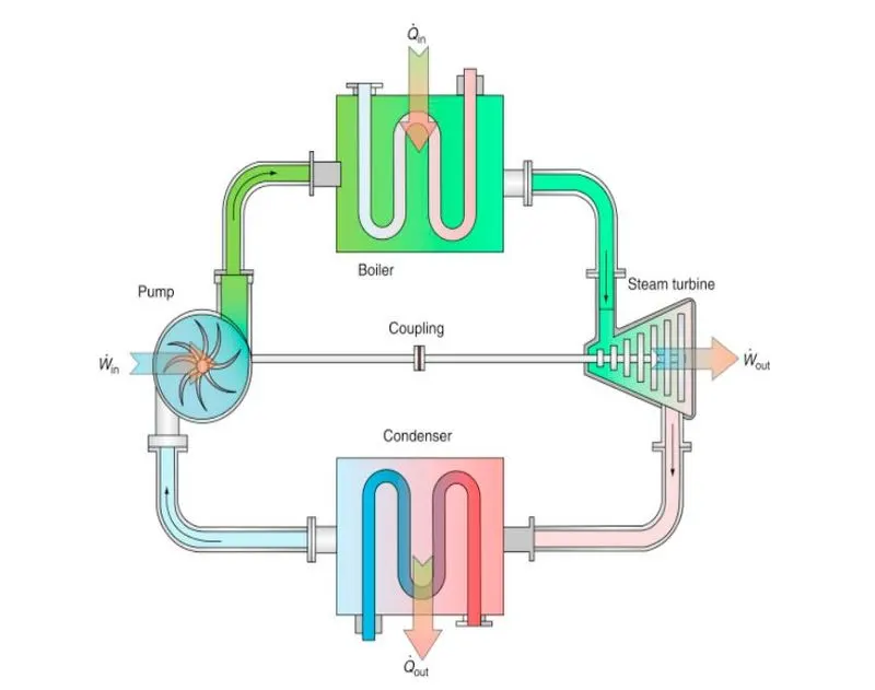
All the four components of rankine cycle are steady flow devices hence the process regarding this devices can be evaluated as steady state process. The steady state energy flow equation per unit mass of steam reduced to,
`(qIn -qOut) +(WIn -WOut) = he-hi`
The boiler and condensor are not involved any mechanical work where as pumps and turbines are assumed to isentropic in nature while working in throughout the cycle then conservation of energy relation for each device can be expressed as
`Wpump = h2-h1`
Where, `h1 = hfatP1 and v1 = vfatP1`
The heat added in boiler can be given as,
`qIn = h3-h2`
The work which can be taken out of cycle from turbine is given as
`Wout = h3-h4`
The removed from the condensor is given by,
`qout = h4-h1`
The thermal efficiency of rankine cycle is given as
`etath = (W Net)/(qIn) = 1-(qOut)/(qIn)`
where,
`WNet = qIn - qOut = Wturb - Wpump`
Code and Explanation :-
clear all
close all
clc

%Rankine Cycle Simulator
fprintf('*Rankine Cycle Simulator*\n\n')
fprintf('Process 1-2 Isentropic Expansion Process\n')
fprintf('Process 2-3 Constant Pressure Heat Rejection Process\n')
fprintf('Process 3-4 Isentropic Compression Process\n')
fprintf('Process 4-1 Constant Pressure Heat Addition Process\n\n\n')

%Required inputs
disp('Inputs required from user side')
T1 = input('Inlet Temperature of Turbine in degree celcius =') ;        %In degree celcius
p1 = input('Pressure at inlet of Turbbe in bars =');                    %In Bars
p2 = input('Outlet pressure of Turbine in bars  =');                    %In Bars

%Extracting Data from Xsteam file for state-1
h1 = XSteam('h_pT',p1,T1);           %Enthalpy at Pressure P1 and Temperature T1
s1 = XSteam('s_pT',p1,T1);           %Entropy at Pressure P1 and Temperature T1

%Extracting Data from XSteam file for state-2
s2 = s1;                            %Because of Isentropic Expansion
% Taking data from Xsteam file for State point 2
s2 = s1;                            % Because of Isentropic Expansion
sf2 = XSteam('sL_p', p2);           % Saturated liquid entropy at pressure 2
sg2 = XSteam('sV_p', p2);           % Saturated vapour entropy at pressure 2
x2 = (s2-sf2)/(sg2-sf2);            % Vapour Fraction at state point 2
hf2 = XSteam('hL_p', p2);           % Saturated liquid Enthalpy at pressure 2
hg2 = XSteam('hV_p', p2);           % Saturated vapour Enthalpy at pressure 2
h2 = hf2 + (x2*(hg2-hf2));          % Enthalpy at state point 2

% Taking data from Xsteam file for state point 3
p3 = p2;                            % Constant Pressure heat removal process
s3 = XSteam('sL_p', p3);            % Saturated liquid entropy at Pressure 3
h3 = XSteam('hL_p', p3);            % Saturated liquid Enthalpy at Pressure 3

% Taking data from Xsteam file for State point 4
s4 = s3;                            % Isentropic Compression process
p4 = p1;                            % Constant Pressure heat rejection

% Work done in Turbine for the rankine cycle
W_T = h1-h2;

% Work done required for pump
v3 = XSteam('vL_p',p3);             % Saturated Liquid Vapour at pressure 3
W_P = v3*(p4-p3)*100;               % Work done for pump
h4 = h3 - W_P;                      % Enthalpy at State point 4

% Net work done for Rankine Cycle
W_net = W_T - W_P;

% Heat Addition to System
Q_in = h1-h4;

% Heat Rejection from System
Q_out = h2-h3;

% Thermal Efficiency of Rankine Cycle
T_eff = (W_net/Q_in)*100;

%specific steam consumption  = (Mass flow rate / Net work done)
Sp_S = (3600/W_net);

% Calculation of Temperature at All state Point 2, 3 and 4
T3 = XSteam('Tsat_p',p3);           % Saturation Temperature at Pressure 3
T2 = T3;                            % Becuase of Constant Pressure Heat addition
Cp4 = XSteam('Cp_ps',p4,s4);        % Specific isobaric heat capacity
Cv4 = XSteam('Cv_ps',p4,s4);        % Specific isochoric heat capacity
k = Cp4/Cv4;
T4 = T3/((p3/p4)^((k-1)/k));        % Temperature at State point 4

% Calculation of Other constant for saturated liquid and Vapour
T6 = XSteam('Tsat_p', p1);          % Saturated Temperature at Pressure 1
s5 = XSteam('sL_p', p1);            % Saturated Liquid entropy at pressure 1
s6 = XSteam('sV_p', p1);            % Saturated Vapour entropy at Pressure 1
h5 = XSteam('hL_p', p1);            % Saturated Liquid Enthalpy at Pressure 1
h6 = XSteam('hV_p', p1);            % Saturated Vapour Enthalpy at pressure 1
T5 = T6;

%Plotting for Saturation Line
T = linspace(1,560,1000);
for i = 1:length(T)
    sf(i) = XSteam('sL_T' ,T(i));   % Saturated Liquid Entropy
    sg(i) = XSteam('sV_T' ,T(i));   % Saturated Vapour Entropy
    hf(i) = XSteam('hL_T' ,T(i));   % Saturated Liquid Enthalpy
    hg(i) = XSteam('hV_T' ,T(i));   % Saturated Vapour Enthalpy

end

% Plotting T-S Diagram for Rankine Cycle
figure(1)
hold on
plot(sf,T,'color','b','linewidth',2)
plot(sg,T,'color','b','linewidth',2)
plot([s1 s2],[T1 T2], 'color', 'r', 'linewidth',3)
plot([s2 s3],[T2 T3], 'color', 'r', 'linewidth',3)
plot([s3 s4],[T3 T4], 'color', 'r', 'linewidth',3)
plot([s4 s5],[T4 T5], 'color', 'r', 'linewidth',3)
plot([s5 s6],[T5 T6], 'color', 'r', 'linewidth',3)
s_1 = linspace(s6,s1,1000);
for j = 1:length(s_1)
    Tc(j) = XSteam('T_ps',p1,s_1(j));
end
plot(s_1,Tc,'color','r','linewidth',3)
text(s1+0.1, T1, '1')
text(s2+0.1, T2, '2')
text(s3, T3-20, '3')
text(s4, T4+20, '4')
title('Temperature Vs Entropy')
xlabel('Entropy (Kj/kg-k)')
ylabel('Temeperature (Deg. Celcius)')
legend('Saturation Curve')

% Plotting H-S Diagram for Rankine Cycle
figure(2)
hold on
plot(sf,hf,'color','b','linewidth',2)
plot(sg,hg,'color','b','linewidth',2)
plot([s1 s2],[h1 h2],'color','r','linewidth',3)
plot([s2 s3],[h2 h3],'color','r','linewidth',3)
plot([s3 s4],[h3 h4],'color','r','linewidth',3)
hc = linspace(h4,h5,100);
for k = 1:length(hc)
    s_c(k) = XSteam('s_ph',p1,hc(k));
end
plot(s_c,hc,'color','r','linewidth',3)
plot([s5 s6],[h5 h6],'color','r','linewidth',3)
for l = 1:length(s_1)
    h_c(l) = XSteam('h_ps',p1,s_1(l));
end
plot(s_1,h_c,'color','r','linewidth',3)
text(s1+0.1,h1,'1')
text(s2+0.1,h2,'2')
text(s3,h3-100,'3')
text(s4,h4+200,'4')
title('Enthalpy Vs Entropy')
xlabel('Entropy (Kj/kg-k)')
ylabel('Enthalpy (KJ/Kg)')
legend('Saturation Curve')

% Displaying Results in Command window
disp('Results of Rankine Cycle')
fprintf('At state point 1\t\t\t\t\t')
fprintf('At state Point 2\n')
fprintf('P1 = %10f in Bar\t\t\t\t',p1);
fprintf('P2 = %10f in Bar\n',p2);
fprintf('T1 = %11f in Deg.Celcius\t\t',T1);
fprintf('T2 = %11f in Deg.Celcius\n',T2);
fprintf('H1 = %12f in KJ/Kg\t\t\t',h1);
fprintf('H2 = %12f in KJ/Kg\n',h2);
fprintf('S1 = %9f in KJ/Kg-k\t\t\t',s1);
fprintf('S2 = %9f in KJ/Kg-k\n',s2);
fprintf('\n')
fprintf('At state point 3\t\t\t\t\t')
fprintf('At state Point 4\n')
fprintf('P3 = %10f in Bar\t\t\t\t',p3);
fprintf('P4 = %10f in Bar\n',p4);
fprintf('T3 = %11f in Deg.Celcius\t\t',T3);
fprintf('T4 = %11f in Deg.Celcius\n',T4);
fprintf('H3 = %12f in KJ/Kg\t\t\t',h3);
fprintf('H4 = %12f in KJ/Kg\n',h4);
fprintf('S3 = %9f in KJ/Kg-k\t\t\t',s3);
fprintf('S4 = %9f in KJ/Kg-k\n',s4);
fprintf('\n')
fprintf('Turbine Work Done = %14f in KJ/Kg\n',W_T)
fprintf('Pump Work Done = %15f in KJ/Kg\n',W_P)
fprintf('Net Work Done  = %17f in KJ/Kg\n',W_net)
fprintf('Thermal Efficiency = %13f in percent\n',T_eff)
fprintf('Sp. Steam Consumption = %f in KJ/Kw\n',Sp_S)
Step-1 :- Generation of Rankine Cycle Simulator. Which requires some inputs from user side for futher calculation of state points at each stage.
Step-2 :- Rankine cycle simulator shows the line command window that Inputs required from user side. Then user has to enter the inputs required, as per given instructions. This inputs are nothing but Inlet turbine temperature, Inlet pressure of turbine and outlet pressure of turbine.
Step-3 :- Then by using XSteam function, state points of stage-1 is extracted. Once we get all values at stage-1 then some values for stage-2 can be calculated based on process, as process2-3 is isentropic compression we can say that entropy will be same i.e. s2 = s1. further state points can be extarcted from XSteam function.
Step-4 :- Similarly state points at stage-3 and stage-4 is extracted from XSteam function.
Step-5 :- Calcualte workdone by turbine with help of enthalpy at stage-1 and stage-2, work done is given by (h1-h2). Then work done by pump need to calculate for this, required saturated vapour at pressure p3. based on that we can calculate work done by pump by (V3*(p4-p3)*100).
Step-6 :- Then heat addition and heat rejection at constant pressure is calculate by using formula Qin=(h1-h4) and Qout=(h2-h3).
Step-7 :- Thermal Efficiency of Rankine cycle is calculated by (Net work done/Heat added in system) and then converted in percentage. Net workdone can be given by (work done by turbine-Work required by pump).
Step-8 :-Then temperature at each stage is calculate by using inputs from start of program and inputs extracted from XSteam function.
Step-9 :-Once we get all the temperatures the next step is to form saturation line using linspace command i.e. T = linspace(1,400,1000) that means it will create from 1 to 400 limit, 1000 points. Which are used for further plotting of graphs.
Step-10 :- At last graphs are plotted for calculated results. Graphs for T-S and H-S are plotted from respective Rankine cycle.
Results :-
Enthapy Vs Entropy i.e. H-S Diagram.
Temperature Vs Entropy i.e. T-S Diagram.
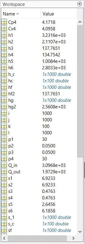
Variables Created in workspace.
Command Window Showing Calculated Results.