Week 3 - Solving second order ODEs

AIM:write a program that solves the following ODE

OBJECTIVE:

• To write a program that solves the ODE that represents the equation of motion of a simple pendulum with damping.
• To animate the motion of the pendulum.

INTRODUCTION:

Concepts & Definition

An ordinary differential equation (ODE) is a diferential equation containing one or more functions of one independent variable and the derivative of those functions.The term ordinary is used in contrast with the term partial differential equation which may be with respect to more than one independent variable.

Here is the ordinary differntial equation that we will be solving:-

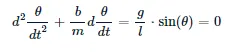
Formulas used:

Consider the following diagram

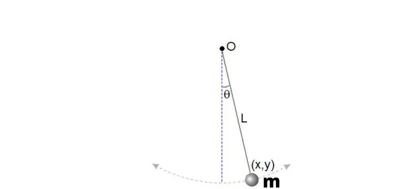
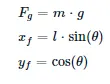
Where;

F_g = Weigth in Newton,

m=mass of the pendulum in Kg,

b = damping coefficient,

xf=length of the projection of the pendulum on X-axis,

yf = length of the projection of the pendulum on y-axis,

Code and explanation

import numpy as np  
from scipy.integrate import odeint
import matplotlib.pyplot as plt
import math

#Function that returns dz/dt 
def model(theta,t,b,g,l,m):
	theta1 = theta[0]
	theta2 = theta[1]
	dtheta1_dt = theta2 
	dtheta2_dt = -(b/m)*theta2 - (g/l)*math.sin(theta1)
	dtheta_dt = [dtheta1_dt,dtheta2_dt]
	return dtheta_dt
b= 0.05
g= 9.81
l= 1
m= 1

#initial condition
theta_0=[0,3]

#Time points 
t = np.linspace(0,20,600)

#Solve ODE
theta = odeint(model,theta_0,t,args = (b,g,l,m))

# Plot results
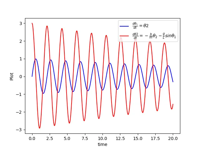
plt.plot(t,theta[:,0],'b-',label=r'$\frac{d\theta_1}{dt}=\theta2$')
plt.plot(t,theta[:,1],'r-',label=r'$\frac{d\theta2}{dt}=-\frac{b}{m}\theta_2-\frac{g}{L}sin\theta_1$') 
plt.ylabel('Plot')
plt.xlabel('time')
plt.legend(loc='best')
plt.show()


ct=1 #Initialization

for i in theta[:,0]:
	#THETA1=theta_0(i)
	x0 = 0
	y0 = 0
    
	xf=(l*math.sin(i))
	yf=-(l*math.cos(i))

	filename = 'imag%05d.png' % ct
	ct=ct+1
        
	#PLOTTING or oscillation of the pendulum
	plt.figure()
	#Plotting the base line of the pendulum or the ceiling
	plt.plot([-0.5 ,0.5],[0,0],linewidth =5,color ='black')
	#Plotting of the bar 
	plt.plot([x0,xf],[y0,yf],linewidth=3,color = 'g')
	#Plotting the ball	
	plt.plot(xf,yf,'o',markersize =20,color ='r')
	plt.xlim([-1.5,1.5])
	plt.ylim([-1.5,1.5])
	plt.title('Animation of Simple pendulum')
	plt.savefig(filename)

Output:

Plot

LINK:

https://youtu.be/VkQZJsfSNUA

RESULT:

Here we have done the simulation of pendulum and it is simple but in real life it can be more complex due to other parameters of the environment but the principle is the same.

Conclusion

Differential Equation applications have significance is in both academic and real life. An equation denotes the relation between two quantity or two functions or two variables or set of variables or between two functions. Differential equation denotes the relationship between a function and its derivatives, with some set of formulas. There are many examples which signifies the use of these equations. Ordinary differential equations applications in real life are used to calculate the movement or flow of electricity, motion of an object (pendulum).