Week 3 - Solving second order ODEs
In the above equation,
g = gravity in m/s2,
L = length of the pendulum in m,
m = mass of the ball in kg,
b=damping coefficient.
Write a program in Matlab\Octave that will simulate the pendulum motion, just like the one shown in the start of this challenge.
use,
L=1 metre,
m=1 kg,
b=0.05.
g=9.81 m/s2.
Simulate the motion between 0-20 sec, for angular displacement=0,angular velocity=3 rad/sec at time t=0.
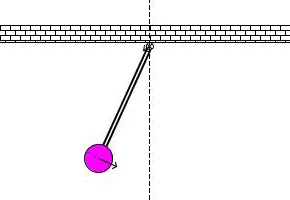
When you do this you will get the position of the pendulum as a function of time. Use this information to animate the motion of the pendulum, as shown in the below figure.
PROGRAM:
A second order differential equation should be converted into single order differential equation. This is done by considering,
θ = θ1
dθ1/dt = θ2
and this leads to following differential equation,
dθ1/dt = θ2
dθ2/dt = -(b/m). θ2 – (g/l). sinθ1
Now these equations can be solved using ode45 function of MATLAB.
The parameters selected for study as follows:
L=1 metre,
m=1 kg,
b=0.05.
g=9.81 m/s2.
With initial conditions,
θ = 0
dθ1/dt = 3
MATLAB MAIN PROGRAM:
% Program to Solve second order ODE for pendulum
clear all
close all
clc
L=1;
m= 0.1;
b=0.05;
g=9.81;
% initial condition
theta_0 = [0;3];
% time points
t_span = linspace(0,20,500);
%solve ODE
[t,results] = ode45(@(t,theta) ode_func (t, theta, b,g,l,m),t_span, theta_0);
plot(t,results(:,1))
hold on
plot(t,results(:,2))
xlabel('time')
ylabel('plot')
% creating animation
Ct = 1;
For i = 1 : length(results(i,1));
x0 = 0;
y0 = 0;
x1 = l*sin(results(i,1));
y1 = l*cos(results(i,1));
figure(2)
plot([-1 1], [0 0], ‘linewidth’, 10 , ‘color’, ‘g’ )
axis([-2 2 -2 2])
hold on
line([x0 x1], [y0 y1], ‘linewidth’, 5 , ‘color’, ‘b’ )
plot(x1 , y1 , ‘markersize’, 25 , ‘markerfacecolor’, ‘r’ )
hold off
M(ct) = getframe(gcf);
Ct = ct+1;
End
%create movie
Movie(M)
videofile = videowriter ('Pendulum_Simulation.avi' , 'uncompressed AVI');
open(videofile);
writevideo(videofile,M)
close(videofile)
ode_function:
function [dtheta_dt] = ode_func (t,theta,b,g,l,m)
theta1 = theta(1)
theta1 = theta(2)
dtheta1_dt = theta2;
dtheta2_dt = -(b/m)*theta2 - (g/l)*sin(theta1);
dtheta_dt = [dtheta1_dt; dtheta2_dt];
end
ode_function converts second order differential equation into two single order differential equations.
Code is explained used comments at each section.
Plots:
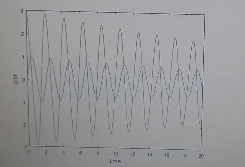
In Plot blue curve represents displacement and red curve represents velocity.