Week 3 - Solving second order ODEs

Program that solves the ODE which represents the equation of motion of a simple pendulum with damping.

given:- damping coefficient,mass of ball,length of string,time span,intial angular velocity ,ODE.

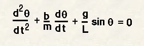
following code is used while solving ODE and stepwise explanation is given.

function [ dtheta_dt ]= ode_func(t,theta,b,g,l,m)% defining function for ode45. 

theta1 =theta(1);                            % assigning first element of theta to theta 1
theta2 = theta(2);                           % assigning secong element of theta to theta 2
dtheta1_dt = theta2;
dtheta2_dt = (-b/m)*theta2-(g/l)*sin(theta1);
dtheta_dt = [dtheta1_dt;dtheta2_dt];         % forming an array of dtheta/dt.

end

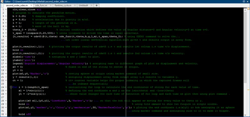
clc,clear,close all
% program to simulate the pendulum motion.
b = 0.05;    % damping coefficient.
g = 9.81;    % acceleration due to gravity in m/s2.
l = 1;       % length of the pendulum in m.
m = 1;       % mass of the ball in kg.
theta_0 = [0;3];             % initial condition which defines the value of Angular distance=0 and Angular velocity=3 at time t=0.
t_span = linspace(0,20,500); % using linspace to divide the time in equal intervals.
[t,results] = ode45(@(t,theta) ode_func(t,theta,b,g,l,m),t_span,theta_0); % using ODE45 command to solve the...
                                ...1st order linear deffrential equation.wich gives t and results output in array form.

plot(t,results(:,1));   % plotting the output results of ode45 i.e t and results 1st coloum i.e time v/s displacement. 
hold on 
plot(t,results(:,2));   % plotting the output results of ode45 i.e t and results 2nd coloum i.e time v/s velocity. 
xlabel('time');         % assigning x and y label to plot.
ylabel('plot');
legend('Angular displacement','Angular velocity'); % assigning name to different graph of plot as displacment and velocity.
x0 = 0;                            % fixed on end of the string to center or origin.
y0 = 0;
plot(x0,y0,'Marker','o')           % creting sphere at origin using marker command of small size.
y = results(:,1);                  % assigning displacement array from output array i.e results to variable y.
ct = 1;                            % ct= counter variable helps for proper indexing in which the captured frames will 
                                     ...be indexed sequentially
for i = 1:length(t_span)           % initializing for loop to calculate the end cordinates of string for each value of time. 
    x1 = l*sin(y(i));              % defining the end cordinate x and y as the lsin(theta) and -lcos(theta)
    y1 = -l*cos(y(i));             ...whose value changes for each time of execution of for loop and each time we plot then using plot command .
                    
    plot([x0 x1],[y0,y1],'LineWidth',3,'Marker','o'); ... so that the bob will appear as moving for every value to theta or y.
    hold on                                                                    % using hold ommand to show two fingure in single window.
    plot(x1,y1,'marker','o','Color','g','markersize',30,'MarkerFaceColor','g'); % ploting the end cordinate i.e(x1y1) or bob assinging it as sphere
                                                                            ...using marker command and assingning size to it to make it bigger.
    hold off
    title({'simple harmonic motion'; 'of a pendulam'},'color','r')% assingning title to plot           
    axis([-1 1 -2 0]);                                            % deffinging axis to make it fixed so that it will not move while running. 
    pause(0.01);                                                  % using plot command to hold the graph for a while 
    xlabel('time');                                               % providing x and y label to graph
    ylabel('angular displacement & angular velocity');
    M(ct)= getframe(gcf);                                         % getframe capture the figure as frame and gcf give current figure to getframe 
    ct=ct+1;                                                      ...to capture and forming the captuerd frame as array and assining it to array M.
end
movie(M);                                                           % play the movie frams in 'M' array ones
videofile = VideoWriter("second_order_odes.avi","Uncompressed AVI");% videowriter will create a video file with specified name and format
open(videofile);                                                    % open video file
writeVideo(videofile,M);                                            % this command enable to create video file with frames captured in 'M' array
close(videofile);                                                   % close video file.

and the function involve is also given

the output of the above programing is the simulated pendulum which can be seen from below given link.

https://www.youtube.com/watch?v=c20CNdEAMHM&ab_channel=GaMeUlTiMaTe