Challenge

Week 3 - Solving second order ODEs

OBJECTIVE:-

Write Code and Describe the transient behavior of a system.

A simple Pendulum.The way the pendulum moves depends on the Newtons second law. When this law is written down, we get a second order Ordinary Differential Equation that describes the position of the "ball" w.r.t time.

THEORY:-

An ordinary differential equation (ODE) is an equation containing an unknown function of one real or complex variable x, its derivatives, and some given functions of x. The unknown function is generally represented by a variable (often denoted y), which, therefore, depends on x.

Simple Pendulum:-The simple pendulum is another mechanical system that moves in an oscillatory motion. It consists of a point mass 'm' suspended by means of light inextensible string of length L from a fixed support.

ODEs EQUATION:-

'd^2(theta)/(dt)+(b/m)*d(theta)/(dt)+(g/l)*sin(theta)=0'
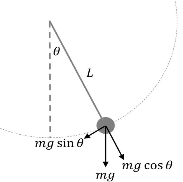
b =damping coefficient,
g = gravity,m/s^2
l=length of rope/string,m
m=mass of ball,kg
GIVEN VALUES:-
b=0.02
g=9.81m/s^2
l=1m
m=0.1 kg
Motion b/w
0-20 sec
angular velocity = 2
angular displacement = 0
interval = 300
EXPLANATION:-
  • Program start with clear all, close all , clc.
  • Derive into values of b,g,l,m with their units.
  • Input of initial condition of angular displacement and angular velocity.
  • For define t_span as 20 second in interval of 300.
  • Always remember when we solve ODE in which we define first ode velocity and displacement.
  • When we solve first order ODEs
  • We will integrated odes system to come into system w.r.t time.
  • ODE is inbuild solver in matlab contain function of (t) and (theta).
  • In ode45(@(t,theta) is dependent and independent variable.
  • And after call ode_func(t,theta,b,g,l,m)
  • First order odes=dtheta1_dt = theta2.
  • Second order odes = dtheta2_dt = -(b/m)*theta2 - (g/1)*sin(theta1).
  • i.e. when we combine in array so we get ,dtheta_dt = [dtheta1_dt; dtheta2_dt].
  • We obtained the result from th function will be 2 coloum of angular displacement and angular velocity w.r.t time.
  • Plot are plotted with the use of function.
  • Use command a for-loop (or simply for loop) is a control flow statement for specifying iteration, which allows code to be executed repeatedly.
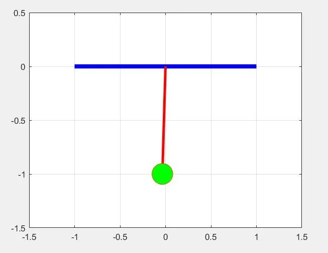
  • 'Markersize' function command is used to make the bob of pendulum circular and 'markerFacecolor' function command is used to color the same.
  • Getframe is used to collect frame and movie function to make movie.
  • To save the video use command = VideoWriter('simple pendulum.avi','Uncompressed AVI')
  • Last generate an avi. file to see th animation video and saved that.

FUNCTION CODE:-

function [dtheta_dt] = ode_func(t,theta,b,g,l,m)
theta1 = theta(1)
theta2 = theta(2)
dtheta1_dt = theta2;
dtheta2_dt = -(b/m)*theta2 - (g/1)*sin(theta1);
dtheta_dt = [dtheta1_dt; dtheta2_dt];
end

FINAL CODE:-

%close all
%clear all
clc
%input
b = 0.02; %damping coefficient
g = 9.81; %gravity
l=1; %length of rope/string
m=0.1; %mass of ball
%initial condition for velocity and displacement
theta_0 = [0;2]; %angular displacement = 0; %angular velocity = 2;
%time interval
t_span = linspace(0,20,300); %generate values from 0 to 20 for 300
%differential equation
[t,results] = ode45(@(t,theta) ode_func(t,theta,b,g,l,m),t_span,theta_0); %ode solver for one degree equation
%plotting
figure(1)
plot(t,results(:,1)) %angular displacement
hold on
plot(t,results(:,2)) %angular velocity
ylabel('angular displacement and angular velocity')
xlabel('time(second)')
title('Damped Harmonic motion of a pendulum')
legend({'displace','velocity'})
grid on
%Creating Animation of simple pendulum
ct = 1;
for i = 1:length(t_span)
THETA = results(i,1);
x0 = 0;
y = 0;
x1 = l*sin(THETA);
y1 = -l*cos(THETA);
figure(2)
plot([-1,1],[0 0],'linewidth',5,'color','b')
line([x0 x1],[y0 y1],'linewidth',3,'Color','r');
hold on
plot(x1,y1,'o','MarkerSize',25,'MarkerFaceColor','g');
grid on
axis([-1.5 1.5 -1.5 0.5]);
pause(0.03);
hold off
M(ct) =getframe(gcf);
ct = ct+1
end
movie(M)
videofile = VideoWriter('simple pendulum.avi','Uncompressed AVI');
open(videofile)
writerVideo(videofile,M)
close(videofile)
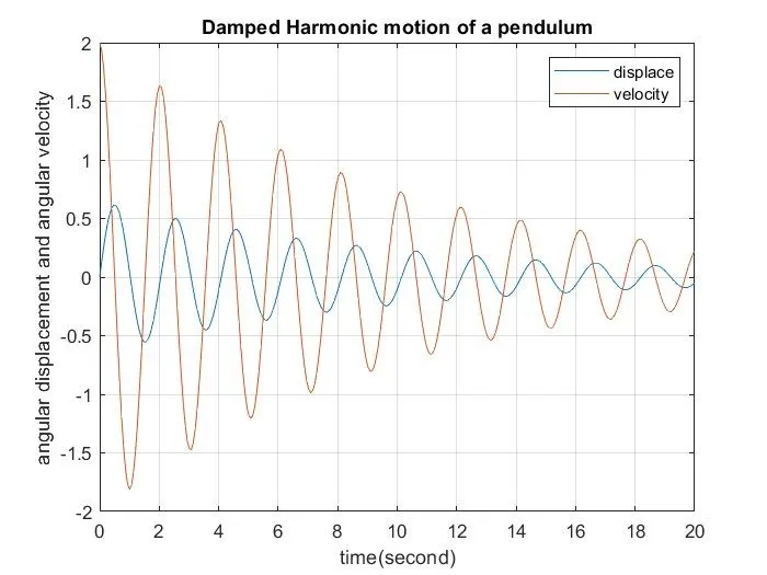
OUTPUT:- Graph of Angular velocity and Angular displacement with respect to time.
  • The amplitude of vibration keeps decreasing as it should in the damped vibration.
  • Objective is achieved.

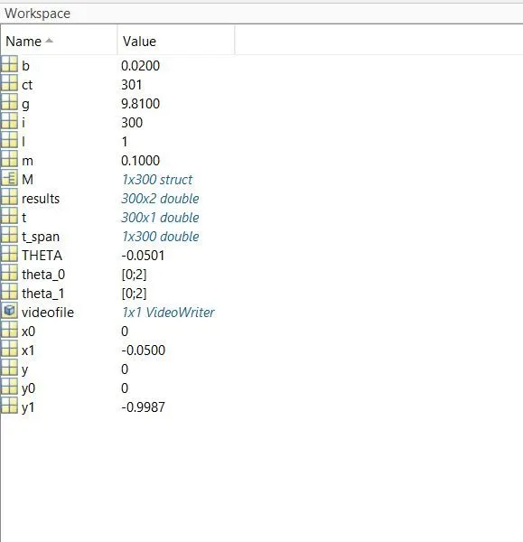
Screen shot of (Animation)
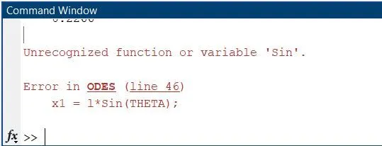
Errors:- Typo error found
  1. Sin is a wrong way to represent , because of upper case
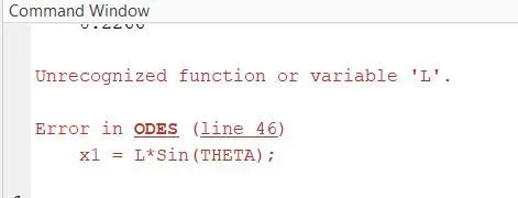
wrote 'Sin' instead of 'sin'
2. upper 'L' is wrong way to represent , because of upper case
wrote 'L' instead of 'l' as per i mentioned
ANIMATION VIDEO
YOUTUBE LINK FOR ODE OUTPUT:
CONCLUSION:-
In graph we see that angular velocity and angular displacement changes with repect to time due to this the effect of damping values changes and reduces with repect to time.
Your portfolio, next

Ship work like this
in your own course.

Talk to a career counsellor

Free 20-minute call. We'll map the right course to where you want to work.

By submitting you agree to our Terms and Privacy Policy.

Talk to a career counsellor

Free 20-minute call. We'll map the right course to where you want to work.

By submitting you agree to our Terms and Privacy Policy.