Week 3 - Solving second order ODEs

Solving second order ODEs

1.AIM:-

To create a MATLAB program that solves the following ODE. This ODE represents the equation of motion of a simple pendulum with damping.

2.OBJECTIVES:-

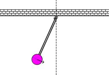
1.Write a program in MATLAB that will simulate the pendulum motion like shown in the

Figure.

2.Upload an animation on YouTube and provide the YouTube link for animation.

3.INTRODUCTION

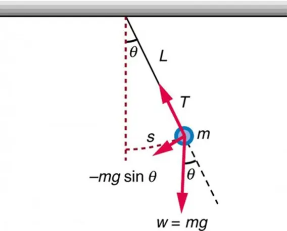
In Engineering, ODE is used to describe the transient behaviour of a system. A simple example is a pendulum. The way the pendulum moves depends on the Newton’s second law. When this law is written down, we get a second order Ordinary Differential Equation that describes the position of the "ball" w.r.t time.

4.PROCEDURE AND EXPLANATION

When a simple pendulum is swung it eventually comes to rest because of gravity and friction. So the equation to calculate will be:

Where:

g = gravity in m/s2,

L = length of the pendulum in m,

m = mass of the ball in kg,

b=damping coefficient.

4.1. Mat lab Program.

1. Program to plot velocity and displacement against time.

Main program.

clear all

close all

clc

%inputs (damping coeff.,gravity,length,mass)

b=0.05;

g=9.81;

l=1;

m=0.1;

%initial conditions

%as initial displacement=0 and initial velocity is 5 m/s

theta_0=[0;5];

%time points

%time array is 0 to 10 seconds with 500 values

t_span=linspace(0,10,500);

%calling ODE function

[t,results]=ode45(@(t,theta)ode_func(t,theta,b,g,l,m),t_span,theta_0)

plot(t,results(:,1),'Color','b')

hold on

plot(t,results(:,2),'Color','g')

xlabel('time')

ylabel('displacement / velocity')

Function program

function[dtheta_dt]=ode_func(t,theta,b,g,l,m)

% defining theta1 and theta2 from the derivation

theta1=theta(1)

theta2=theta(2)

dtheta1_dt=theta2;

dtheta2_dt=-(b/m)*theta2-(g/l)*sin(theta1);

dtheta_dt=[dtheta1_dt;dtheta2_dt]

end

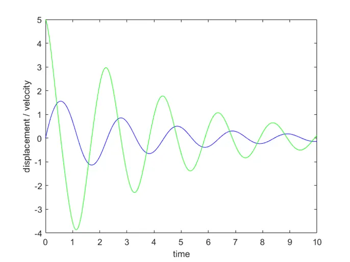
Output

Final main program to write video to a video file.

clear all

close all

clc

%inputs (damping coeff.,gravity,length,mass)

b=0.05;

g=9.81;

l=1;

m=0.1;

%initial conditions

%as initial displacement=0 and initial velocity is 5 m/s

theta_0=[0;5];

%time points

%time array is 0 to 10 seconds with 500 values

t_span=linspace(0,10,500);

%calling ODE function

[t,results]=ode45(@(t,theta)ode_func(t,theta,b,g,l,m),t_span,theta_0)

figure(1)

plot(t,results(:,1),'Color','b')

hold on

plot(t,results(:,2),'Color','g')

xlabel('time')

ylabel('displacement / velocity')

%program to make animation of the simple pendulam

ct=1;

theta_0=results(:,1)

for i=1:length(results(:,1))

x0=0;

y0=0;

theta_1=theta_0(i);

x1=l*sin(theta_1);

y1=-l*cos(theta_1);

figure(2)

%plot of pendualm line from origin

plot([x0 x1],[y0 y1],'linewidth',3,'Color','b')

hold on

%plot of pendulam end point

plot(x1,y1,'.',MarkerSize=30)

%plot of pendulam origin

plot(x0,y0,'.',MarkerSize=50,MarkerFaceColor='r',MarkerEdgeColor='g')

hold off

axis([-1 1 -1.1 0.1])

pause(0.01)

M(ct)=getframe(gcf);

ct=ct+1

end

%to save videofile

movie(M);

videofile=VideoWriter('pendulam.avi','Uncompressed AVI')

open(videofile)

writeVideo(videofile,M)

close(videofile)

Errors occurred during the programming.

1. Error.

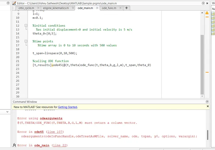
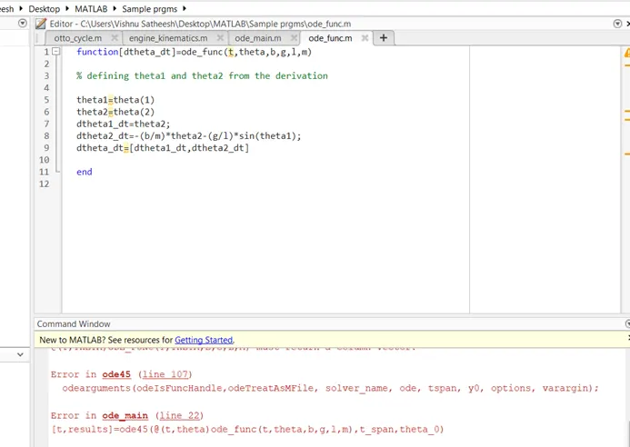
Solution : put semi colon in line no 9 of function program instead of colon.

2. Only velocity plot is coming. Displacement plot was missing.

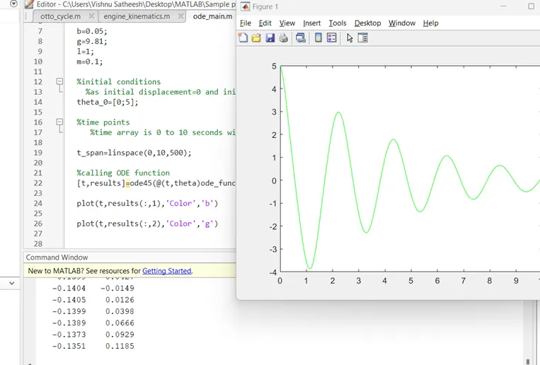
Solution : Added hold on command in between the two plot commands.

3. Plot for pendulum motion was coming like in picture.

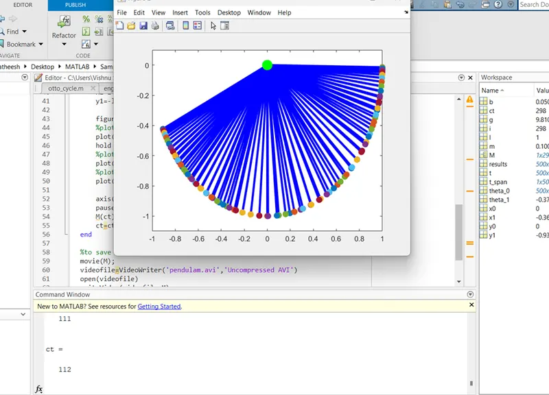
Solution : Added hold off command after the plot commands.

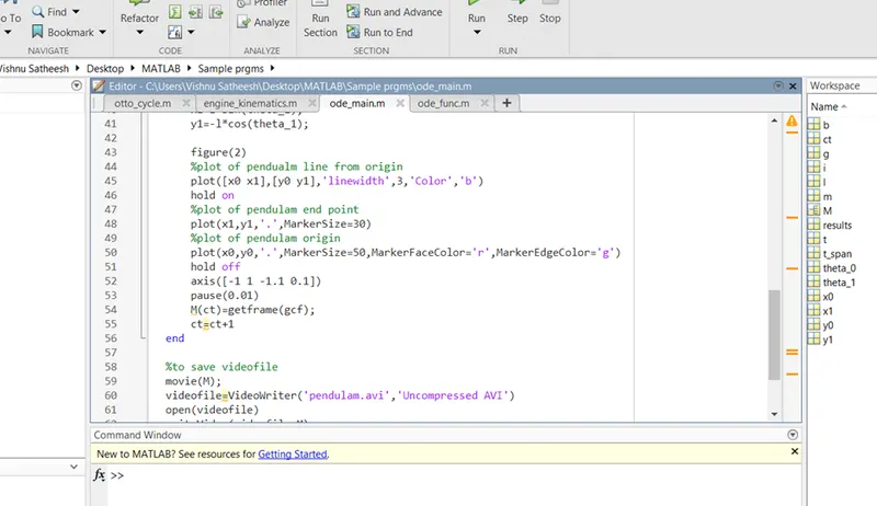
Main program

clear all
close all
clc

%inputs (damping coeff.,gravity,length,mass)

b=0.05;
g=9.81;
l=1;
m=0.1;

%initial conditions
  %as initial displacement=0 and initial velocity is 5 m/s
theta_0=[0;5];

%time points
   %time array is 0 to 10 seconds with 500 values

t_span=linspace(0,10,500);

%calling ODE function
[t,results]=ode45(@(t,theta)ode_func(t,theta,b,g,l,m),t_span,theta_0)

figure(1)
plot(t,results(:,1),'Color','b')
hold on
plot(t,results(:,2),'Color','g')
xlabel('time')
ylabel('displacement / velocity')

%program to make animation of the simple pendulam

ct=1;
theta_0=results(:,1)
for i=1:length(results(:,1))
    x0=0;
    y0=0;

    theta_1=theta_0(i);
    x1=l*sin(theta_1);
    y1=-l*cos(theta_1);

    figure(2)
    %plot of pendualm line from origin
    plot([x0 x1],[y0 y1],'linewidth',3,'Color','b')
    hold on 
    %plot of pendulam end point
    plot(x1,y1,'.',MarkerSize=30)
    %plot of pendulam origin
    plot(x0,y0,'.',MarkerSize=50,MarkerFaceColor='r',MarkerEdgeColor='g') 
    hold off
    axis([-1 1 -1.1 0.1])
    pause(0.01)
    M(ct)=getframe(gcf);
    ct=ct+1
end

Function Program

function[dtheta_dt]=ode_func(t,theta,b,g,l,m)

% defining theta1 and theta2 from the derivation

theta1=theta(1)
theta2=theta(2)
dtheta1_dt=theta2;
dtheta2_dt=-(b/m)*theta2-(g/l)*sin(theta1);
dtheta_dt=[dtheta1_dt;dtheta2_dt]

end