Week 2- 2R Robotic Arm Challenge

FORWARD KINEMATICS OF A 2R ROBOTIC ARM

1. AIM:-

Write a program to simulate the forward kinematics of a 2R Robotic arm.

2. OBJECTIVES:-

• To simulate forward kinematics of a 2R robotic arm.
• To write the simulated part to a video file format

3. INTRODUCTION

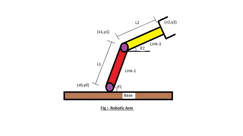
A robotic arm is a type of mechanical arm, usually programmable, with similar functions to a human arm. The links of such a manipulator are connected by joints allowing either rotational motion or translational (linear) displacement. So basically the combinations of such linkages forms a machine.

In the ongoing project it has a two rotating links (2R means two rotational links) as shown in the given figure.

4. PROCEDURE AND EXPLANATION

4.1. Finding position of the link 1.

From the given figure, the initial position of the link is calculated as (0, 0). So coordinates of the end position must be

x1=l1 cosѲ1

y1=l1 sin Ѳ1

4.2. Finding position of the link 2.

The initial position of the link 2 is same as the end point of the link1. The end position must be

x2=x1+l2 cosѲ2

y2=y1+l2 sinѲ2

4.3. Mat lab Program.

Basic Program

% FORWARD KINEMATICS OF A 2R ROBOTIC ARM

close all

clear all

clc

% INPUTS

%Length and angles

l1=1;

l2=0.5;

theta1=30;

theta2=45;

%coordinates of the links

x0=0;

y0=0;

x1=l1*cosd(theta1)

y1=l1*sind(theta1)

x2=x1+l2*cosd(theta2)

y2=y1+l2*sind(theta2)

%plotting

line([x0 x1],[y0 y1],'linewidth',3,'color','b')

line([x1 x2],[y1 y2],'linewidth',3,'color','r')

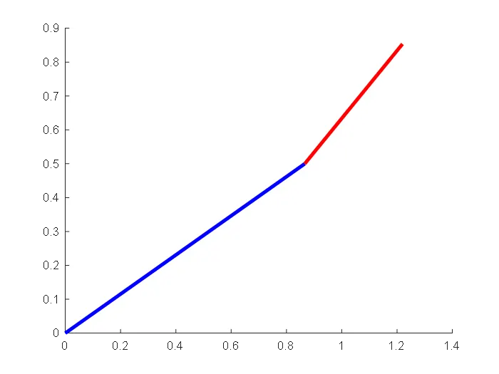
output

x1 =

0.8660

y1 =

0.5000

x2 =

1.2196

y2 =

0.8536

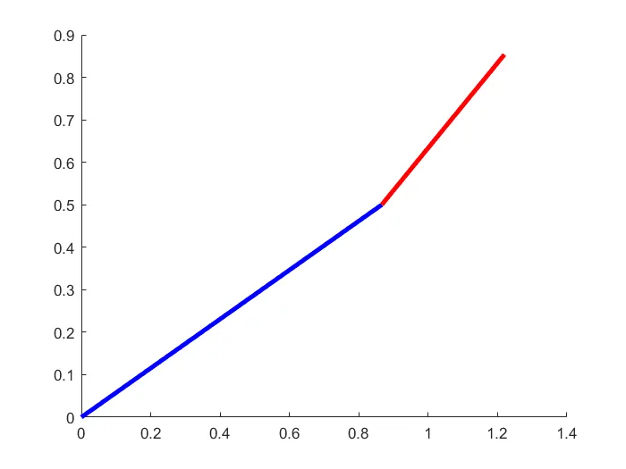
Program for set of angles.

In this we are assigning different variables to Ѳ1 and Ѳ2 to obtain using linspace command and for loop.

In this linspace command the first value represents first angle and second value represents the final angle and third value represents no of angles.

In the loop, the value of i is used to take a particular value theta 1,and the value of j is used to take a particular value for theta2. So for a particular position of link 1, link 2 can take multiple positions.

clear all

close all

clc

%inputs

l1=1;

l2=0.5;

theta1=linspace(0,90,3);

theta2=linspace(0,90,3);

ct=1

for i=1:length(theta1)

THETA1=theta1(i);

for j=1:length(theta2)

THETA2=theta2(j);

x0=0;

y0=0;

x1=l1*cosd(THETA1);

y1=l1*sind(THETA1);

x2=x1+l2*cosd(THETA2);

y2=y1+l2*sind(THETA2);

%plotting

figure(ct)

hold on

line([x0 x1],[y0 y1],'linewidth',3,'color','b')

line([x1 x2],[y1 y2],'linewidth',3,'color','r')

ct=ct+1;

end

end

output

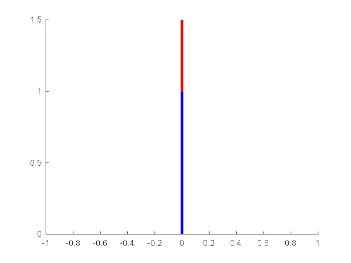
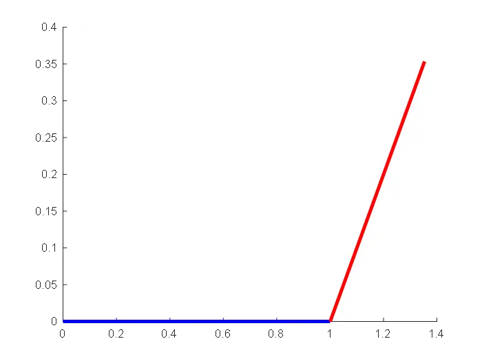
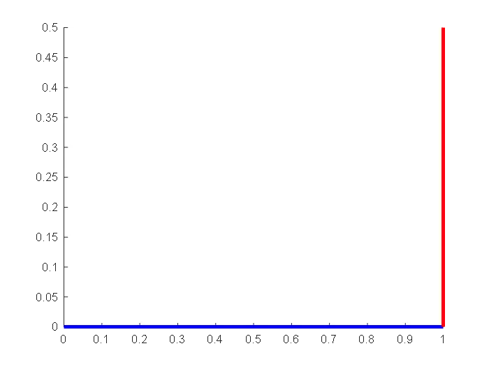
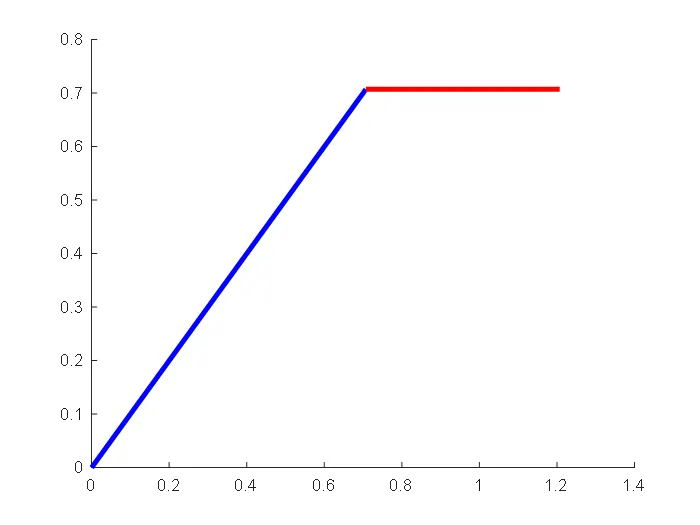
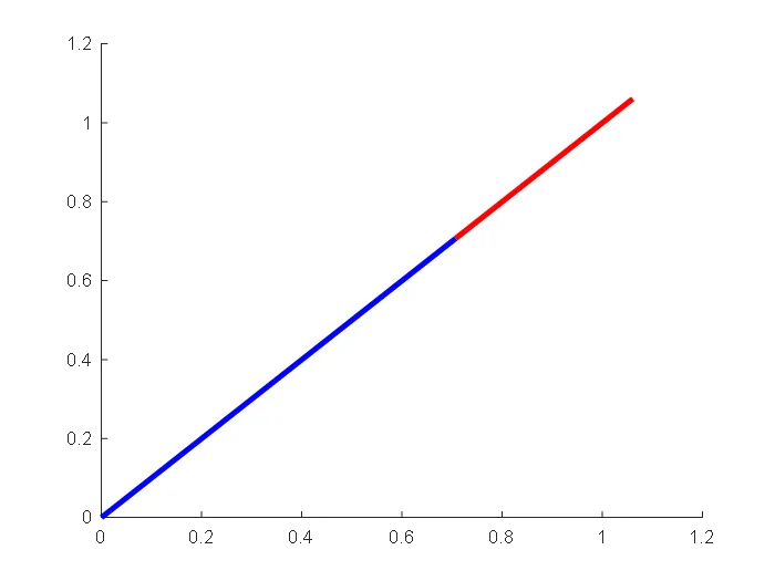
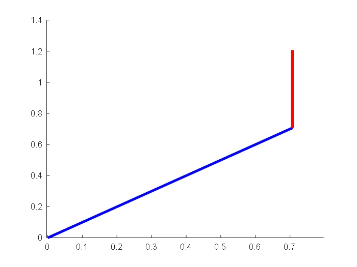
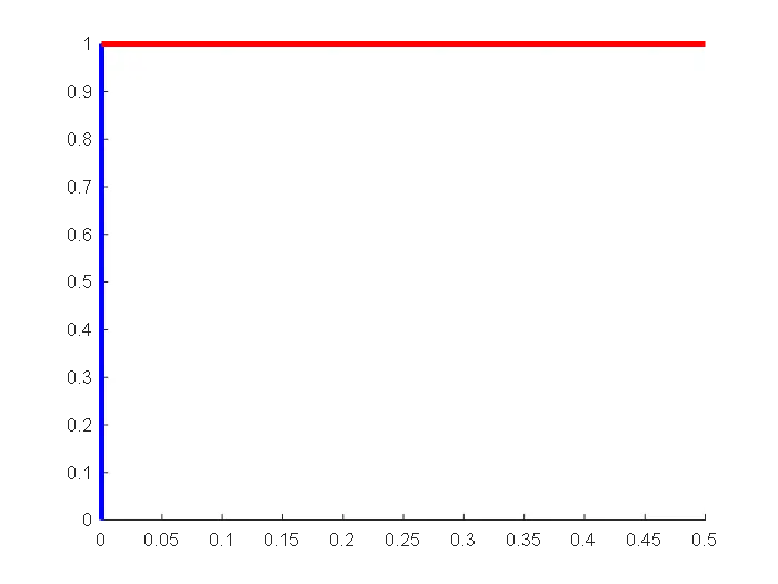
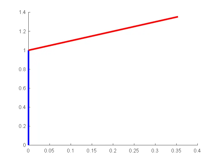
These are the nine output plots that we have got for different set of values for theta1 and theta2. This plots are difficult to identify and also we needed it in a same plot, we have to change some parameters in the programme. That is we have to add a pause of 0.3 seconds to the plotting command section and remove the figure (ct) also to get the plot in a single window in an animated view.

Change in program.

%plotting

hold on

plot([x0 x1],[y0 y1],'linewidth',3,'color','b')

plot([x1 x2],[y1 y2],'linewidth',3,'color','r')

ct=ct+1;

pause(0.3)

end

end

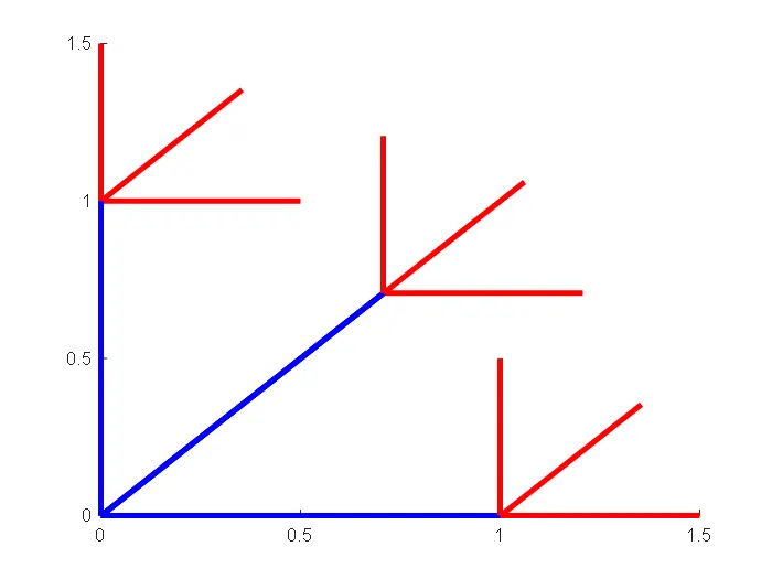
Still the result need more clarity and an animated video we have to continue to change the program in the following way to the plotting session. they are:

1. Remove the second plot command and add it to single command.
2. Remove hold on command
3. Add limits for the axis’s.
4. Reduce pause interval for a better visual effect.

%plotting

plot([x0 x1],[y0 y1],[x1 x2],[y1 y2],'linewidth',3)

axis([-0.1 1.5 0 1.5])

ct=ct+1;

pause(0.1)

end

end

Final program to write the video file

1. Add M(ct) in which ct represents contour or each frame and getframe(gcf) which is the command to get current figure.
2. Add the commands for writing the video to a video file.
3. For a better video experience increase the values in linspace command from 4 to 10.

clear all

close all

clc

%inputs

l1=1;

l2=0.5;

theta1=linspace(0,90,10);

theta2=linspace(0,90,10);

ct=1

for i=1:length(theta1)

THETA1=theta1(i);

for j=1:length(theta2)

THETA2=theta2(j);

x0=0;

y0=0;

x1=l1*cosd(THETA1);

y1=l1*sind(THETA1);

x2=x1+l2*cosd(THETA2);

y2=y1+l2*sind(THETA2);

%plotting

plot([x0 x1],[y0 y1],[x1 x2],[y1 y2],'linewidth',3)

axis([-0.1 1.5 0 1.5])

pause(0.03)

M(ct)=getframe(gcf);

ct=ct+1;

end

end

movie(M);

videofile=VideoWriter('forward_kinematics.avi','Uncompressed AVI');

open(videofile)

writeVideo(videofile,M)

close(videofile)

Various screenshots of simulated video.

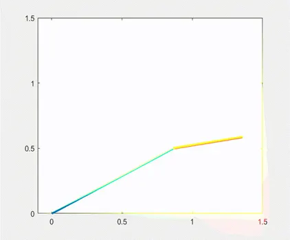
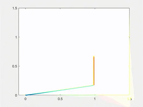
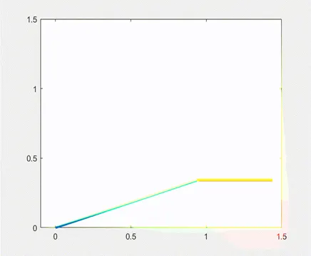
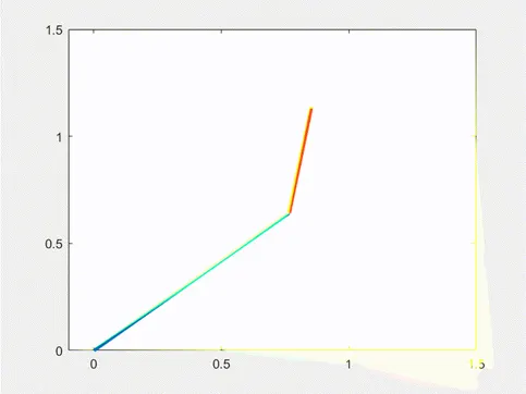
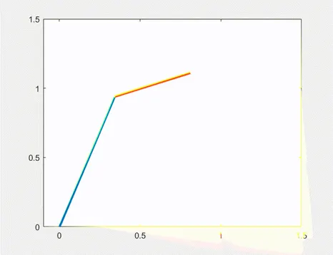
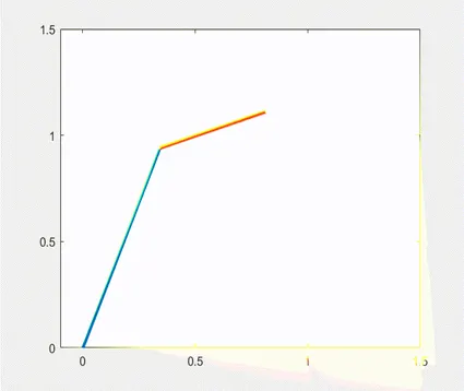
Errors occurred during the programming.

1. Found a wrong plot in the first program as shown in the figure.

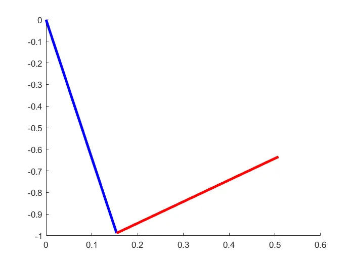
Solution : I identified the mistake that i didn’t added the letter ‘d’ in the cos and sin inputs. After adding i could fint the exact plot.

1. 

1. Forget to provide end to the loop which has two for loop inputs

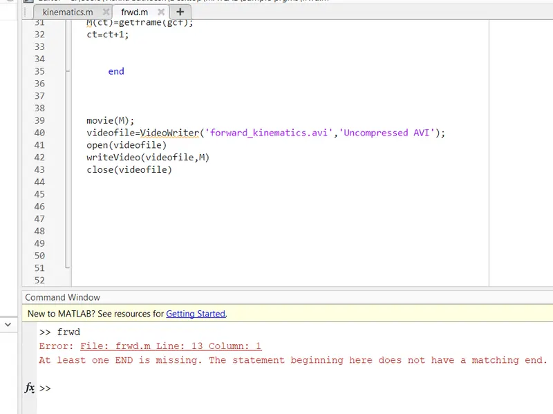
Solution: Identified the mistake that i have to add one more end to the for loop section.

5.RESULT

The video link for the Forward kinematics for a 2R robotic arm

https://youtu.be/5Mf0ZqURA-8

clear all
close all
clc

%inputs

l1=1;
l2=0.5;
theta1=linspace(0,90,10);
theta2=linspace(0,90,10);

ct=1
for i=1:length(theta1)
    THETA1=theta1(i);
    for j=1:length(theta2)
        THETA2=theta2(j);
        x0=0;
        y0=0;

        x1=l1*cosd(THETA1);
        y1=l1*sind(THETA1);

        x2=x1+l2*cosd(THETA2);
        y2=y1+l2*sind(THETA2);

%plotting

plot([x0 x1],[y0 y1],[x1 x2],[y1 y2],'linewidth',3)
axis([-0.1 1.5 0 1.5])
pause(0.03)
M(ct)=getframe(gcf);
ct=ct+1;


    end
end

movie(M);
videofile=VideoWriter('forward_kinematics.avi','Uncompressed AVI');
open(videofile)
writeVideo(videofile,M)
close(videofile)