Week 3 - Solving second order ODEs

PROGRAM SOLVING SECOND ORDER ODE

AIM : The objective is to write a code that solves second order Ordinary Differential Equation and presenting the results by plotting them.

• Here, we will code a program that shows harmonic motion of a pendulum. The ODE for a simple ependulum is given by

• This equation shows the position of the ball(mass) with respect to time as a variable. To solve this second order ODE, first convert it into two first order equations. As you can see in function code, theta is taken as theta1 and derivative of theta1 w.r.t. time is taken as theta2. 
• We now have two equations and the derivative of theta can be written as matrix of other two defined derivatives.
• Create a function with needed inputs.

FUNCTION CODE

function [dtheta_dt] = ode_func(t,theta,b,g,L,m)

theta1 = theta(1);
theta2 = theta(2);
dtheta1_dt = theta2;
dtheta2_dt = -(b/m)*theta2 - (g/L)*sind(theta1);

dtheta_dt = [dtheta1_dt;dtheta2_dt];

end

• As inputs, we are provided with mass, length of pendulum, damping coefficient, gravitational acceleration, initial angular velocity and have to present the motion for time interval of 20 seconds.
• Use the ode45 command and put inputs. Keep ode45 as the funtion of time and angular displacement as variables.
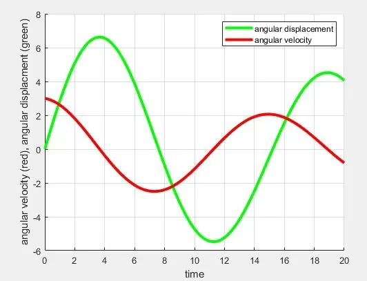
• By this we will get a set of angular displacement and angular velocity.
• Plot them versus time and a result as figure1 will be achieved.
• Now, lets create an animation for pendulum. For this, use a 'for loop' command for the given interval of time.
• To demonstrate a pendulum, assume a hinged end to a rigid body and a ball at another end.
• As it can be seen in the code, marker command is used to present the ball. Colours and size is individual's choice.
• Make sure to use 'hold on' after plotting the rod and 'hold off' after plotting the ball. This will plot both the parts together for one iteration, then erase all and create new pair for new iteration.
• Create a gif out of it by using video writing codes as shown. Link for the video is given below.

MAIN CODE

% A program to simulate a pendulum motion

clear all
close all
clc

% Inputs

% damping coeeficient
b = 0.05;
% mass in kg
m = 1;
% length of pendulum in m
L = 1;
% gravitational acceleration in m/s^2
g = 9.81;

% Initial condition t=0
theta_0 = [0;3];

% time span
t_span = linspace(0,20,500);

% ODE solution
[t,results] = ode45(@(t,theta) ode_func(t,theta,b,g,L,m),t_span,theta_0);


% Plotting

figure(1)
hold on
plot(t,results(:,1),'LineWidth',3,'Color','g')
plot(t,results(:,2),'LineWidth',3,'Color','r')
axis ([0 20 -6 8])
xlabel time
ylabel ('angular velocity (red), angular displacment (green)')
legend('angular displacement','angular velocity')
grid on



% Animation of pendulum

ct=1;
figure(2)

for i = 1:length(t_span)
    x0 = 0;
    y0 = 0;
    x1 = L*sind(results(i,1));
    y1 = -L*cosd(results(i,1));
    
    plot([x0 x1],[y0 y1],[-0.05 0.05],[0 0],'LineWidth',3,'Color','b')
    hold on
    plot(x1,y1,'Marker','o','MarkerSize',30,'MarkerFaceColor','r','MarkerEdgeColor','b')
    axis ([-0.15 0.15 -1.2 0.2])
    
    pause(0.0000001)
    hold off
    M(ct) = getframe(gcf);
    ct=ct+1;

end

% Creating gif
movie(M)
videofile = VideoWriter ('ode_func.avi','Uncompressed AVI')
open(videofile)
writeVideo(videofile,M)
close(videofile)

GRAPH

VIDEO LINK : https://youtu.be/bn5bQDkGO44