Week 3 - Solving second order ODEs

Project Report:
Step1 : Declaring the input variables
Values of Damping coefficient, Acceleration due to gravity, Length of the string and Mass of the pendulum bob is defined.
Step2: Defining the initial condition and time span
Initial condition is defined as 'theta_0 = [0;3]' which implies that at time t = 0, angular velocity is 3 rad/sec.
500 time instant is considered between 0 and 20 seconds by using the command 't_span = linspace(0,20,500)'.
Step3 : Solving the ODE
In the command '[t, results] = ode45(@(t,theta) ode_function(t, theta,b,g,l,m),t_span, theta_0);'
ode45(@(t,theta): This syntax is used to call the inbulit ODE solver in matlab and define the dependent and independent variables in the ODE. Here, time is the independent variable and angualr displacement (theta) is the dependent variable.
ode_function(t, theta,b,g,l,m): This syntax is used to define the ODE function and the variables involved in that function. This function is seperately coded and called by the command 'ode_function'.
t_span, theta_0: This syntax is used to specify the initial condition used to solve the ODE and the time instants between a particular time interval.
Step4 : Plotting the results
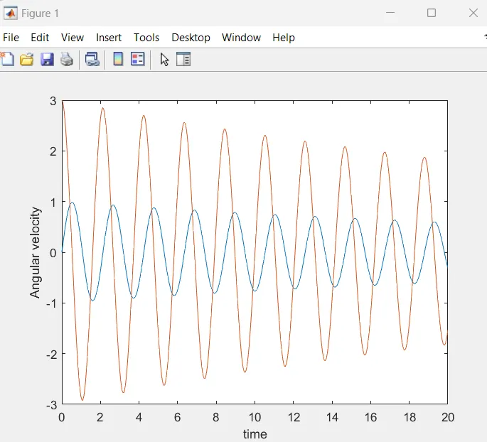
Results are plotted considering time on x axis and angular velocity on y axis.
Step5 : Animation of the motion of the pendulum
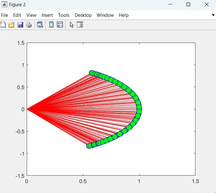
500 time instants are extracted by the command 'results(:,1)' and stored inside a new variable array'theta'. One end of the string is fixed at origin by the command x0=0; y0=0; and other end of the string moves according to the solution of the ODE. This is possible by using the 'for loop'. For loop is intiated from i=1 to length of the variable array 'theta'. Therefore, second end of the string assumes different positions according to the solution of ODE.
Plotting of the pendulum bob:
Pendulum bob is plotted at the end point (x1,y1) of the string by using the marker command.
Step6 : Creating the movie of animation
A Movie of the animation is created by capturing each time frame in the variable M(ct)

clear all

close all

clc

%Step1: Declaring the input variables

b = 0.05; %damping coefficient

g = 9.81; %Acceleration due to gravity

l = 1; %Length of the string

m = 1; %Mass of the pendulum bob

%Step2: Defining the initial condition and time span

%intial condition

theta_0 = [0;3];

%time points

t_span = linspace(0,20,500);

%Step3 : Solving ODE

[t, results] = ode45(@(t,theta) ode(t, theta,b,g,l,m),t_span, theta_0);

%Step4 : Plotting the results

figure(1)

plot(t,results(:,1))

hold on

plot(t,results(:,2))

xlabel('time')

ylabel('Angular velocity')

%Step 5: Animation of the motion of the pendulum

figure(2)

%Saving the values of time in an array variable 'theta'

theta = results(:,1);

ct = 1;

for i = 1:length(theta)

a = theta(i);

x0=0;

y0=0;

x1= l*cos(a);

y1= -l*sin(a);

plot([x0 x1],[y0 y1],'color','r')

hold on

%pendulum bob plot

plot(x1,y1,'O','markersize',10,'color','b','MarkerFaceColor','g');

axis([0 1.5 -1.5 1.5])

pause(0.03);

M(ct) = getframe(gcf);

ct = ct+1;

end

% Step6 : Creating the movie of animation

movie(M)

videofile=VideoWriter('ODE_Pendulum.avi','Uncompressed AVI');

open(videofile)

writeVideo(videofile,M)

close(videofile)