Week 3 - Solving second order ODEs
To write a program to simulate the transient behaviour of simple pendulum and to create an
animation of its motion.
In engineering, ODE is used to describe the transient behaviour of a system. A simple example
is a pendulum. The way the pendulum moves depends on the Newtons second law. When this law
is written down, we geta second order ordinary differential equation that describes the position of
"ball" w.r.t.time.
Similarly, there are hundred of ODEs that describe key phenomena and if you have the ability to solve
these equations then you will be able to the simulate any of these systems.
The governing equation is,
d2θ/dt2+b/m⋅dθ/dt+g/L⋅sinθ=0
In the above equation,
g = gravity in m/s2,
L = length of the pendulum in m,
m = mass of the ball in kg,
b=damping coefficient.
Given,
L=1 metre,
m=1 kg,
b=0.05.
g=9.81 m/s2.
Simulate the motion between 0-20 sec
for angular displacement=0
angular velocity=3 rad/sec
at time t=0.
PROGRAM :-
import numpy as np
from scipy.integrate import odeint
import matplotlib.pyplot as plt
import math
# function that returns d2/dt
def model (theta, t, b, g, l, m):
theta1 = theta[0]
theta2 = theta[1]
dtheta1_dt = theta2
dtheta2_dt = (-b/m)*theta2 - (g/l)*math.sin(theta1)
dtheta_dt = [dtheta1_dt, dtheta2_dt]
return dtheta_dt
# Inputs
b = 0.05
g = 9.81
l = 1
m = 1
# Initial conditions
theta_0 = [0,3]
# time points
t = np.linspace(0,20,200)
# solve ODE
theta = odeint(model, theta_0, t, args = (b, g, l, m))
# plot results
plt.plot(t,theta[:,0])
plt.plot(t,theta[:,1])
plt.ylabel('plot')
plt.xlabel('time')
plt.show()
# Inputs
x0 = 0
y0 = 0
# Animation
ct = 1
y = theta[:,0]
for i in y:
x1 = l*math.sin(i)
y1 = -l*math.cos(i)
filename = str(ct) + '.png'
ct = ct + 1
plt.figure()
plt.plot([-1,1],[0,0],"black", linewidth = 5)
plt.plot([x0,x1],[y0,y1],"red", linewidth = 3)
plt.plot(x1,y1,'o', markersize = 8)
plt.xlim([-1,1])
plt.ylim([-1.5,1])
plt.savefig(filename)
EXPLANTIONS:-
In this python program we used import module numpy as np, scipy.integrate
import odient for second ode, math and for plots matplotlib.
This module we used for importing required modules using 'import' command.
Then we used define function that function model is created with required arguments,
inside which the term which are broken to solve second order ODE are calculated.
Inputs are provided for the function. Initialize the inputs values of b, g, l, m.
Then we took theta_0 ranges between 0 to 3.
After that we used np.linspace for creating numeric sequence it means that np.linspace(
start point, last point, number values take in between start and end point).
Then we used odeint function command. This is used to solve ode function.
After that we used plot result by using plt.plot command to plot graph.
Then we created animation use for loop command. In this for loop command
open a for loop, ranging from 0 to length of t.
Then give name filename.
After that images are saved using savefig command.
Then all the plots to create every single point after that stiches all the pic and create a gif.
OUTPUT:-
RESULTS:-
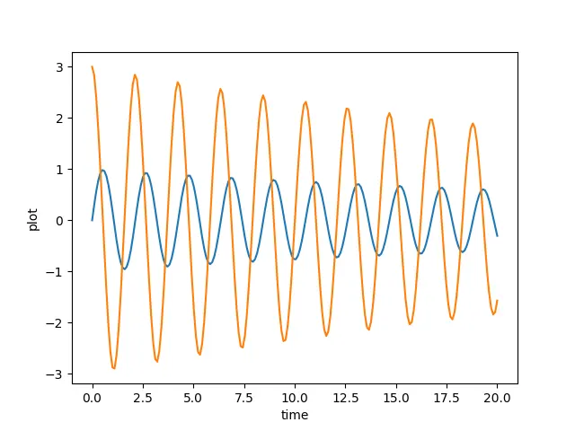
In this graph blue line denoted as displacement and red line denoted as velocity.
Angular displacement and angular velocity with respect to time.
From the graph the values of angular displacement and angular velocity keeps on decreasing
with time, this effect is known as damping effect.
ANIMATION VIDEO LINK:-