Week 3 - Solving second order ODEs

Aim:

Write a program that solves the following ODE. This ODE represents the equation of motion of a simple pendulum with damping

Write a program in MatlabOctave that will simulate the pendulum motion.

Simulate the motion between 0-20 sec, for angular displacement=0,angular velocity=3 rad/sec at time t=0.

use,

L=1 metre

m=1 kg

b=0.05

g=9.81 m/s^2

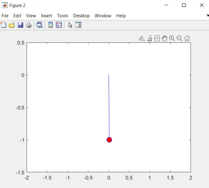
When you do this you will get the position of the pendulum as a function of time. Use this information to animate the motion of the pendulum.

Theory:

In Engineering, ODE is used to describe the transient behavior of a system. A simple example is a pendulum

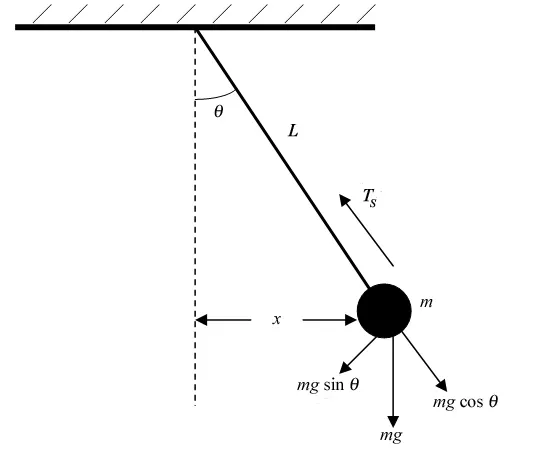
The way the pendulum moves depends on the Newtons second law. When this law is written down, we get a second order Ordinary Differential Equation that describes the position of the "ball" w.r.t time.

The second order ode of simple pendulum is defind as

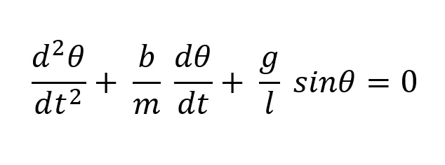
where,

g = gravity in m/s2,

L = length of the pendulum in m,

m = mass of the ball in kg,

b=damping coefficient.

Now breaking down the 2nd order ode into two 1st order ode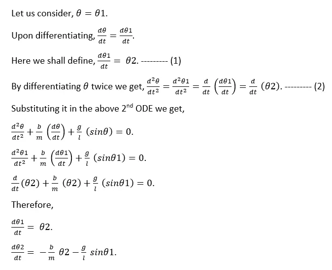

Now we have defined θ1 and θ2.

## Code for solving the 2nd order ode of simple pendulum and simulating it ##

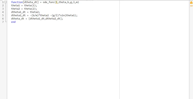
% First the code of the function

function[dtheta_dt] = ode_func(t,theta,b,g,l,m)             % output of the function is dθ/dt
theta1 = theta(1);                                                       % θ1
theta2 = theta(2);                                                       % θ2
dtheta1_dt = theta2;                                                   % dθ1/dt = θ2
dtheta2_dt = -(b/m)*theta2 -(g/l)*sin(theta1);
dtheta_dt = [dtheta1_dt;dtheta2_dt];                          % dθ/dt = [dθ1/dt; dθ2/dt]
end

% Given values

% b=0.05
% g=9.81 m/s^2
% l=1 m
% m=1 kg

% Main Code for ode

% Solving 2nd order ode functions

clear all
close all
clc​

% inputs

b = 0.05;
g = 9.81;
l = 1;
m = 1;​

% initial condition

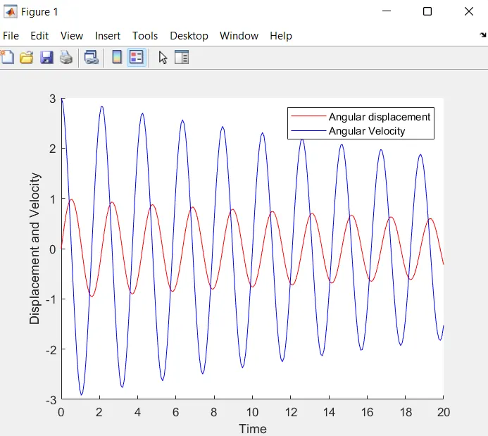
% We have two initial conditions, one for angular displacement and one for angular velocity

theta_0 = [0;3];                    % 0 is for displacment and 3 is for velocity

% time between 0 to 20 sec

t_span = linspace(0,10,250);

% solving of ode

% calling the ode45 functions for different values of time (t_span) and initial conditions (theta_0)

% @(t,theta) refers that the ode function is the function of t and theta

% ode45 is the inbuilt function which outputs t and result

% t is times that result is given

% reslut is output of the function i.,e displacement and velocity

% we have angular displacement and angular velocity at times t

[t,result] = ode45(@(t,theta) ode_func(t,theta,b,g,l,m),t_span,theta_0);

% Graph

hold on
plot(t,result(:,1))
plot(t,result(:,2))
xlabel('Time')
ylabel('Displacement and Velocity')
legend('Angular displacement','Angular Velocity')​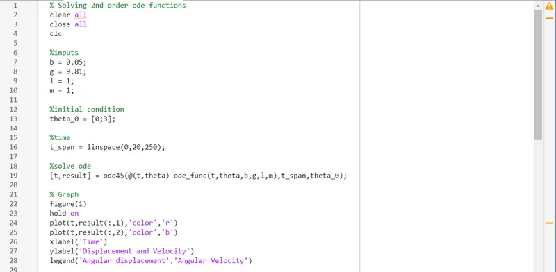

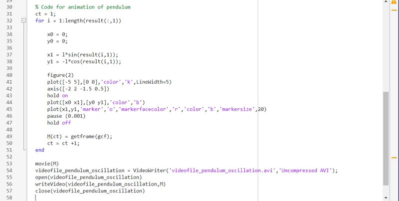
% Code for animation of pendulum

% counter for counting the iteration and saving the frames for the movie in M

ct = 1;

% creat a for loop from 1 to length of the times of result

for i = 1:length(result(:,1))

% co ordinates for the fixed point of the pendulum

x0 = 0;
y0 = 0;
​

% co ordinates for the swinging point of the pendulum fixed to the mass

x1 = l*sin(result(i,1));
y1 = -l*cos(result(i,1));​

% stucture of pendulum

figure(2)
plot([-5 5],[0 0],'color','k',LineWidth=5)               % fixed support
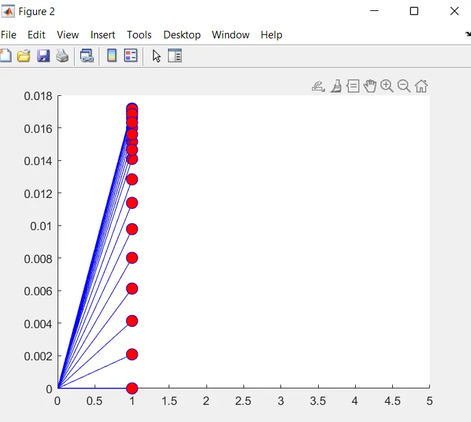
axis([-2 2 -1.5 0.5])      % specifying the axis so it does not move for diffrent frames

hold on
plot([x0 x1],[y0 y1],'color','b')            
plot(x1,y1,'marker','o','markerfacecolor','r','color','b','markersize',20)
pause (0.001)
hold off​

% store all the frames in M by getframe(gct) coomand

% advance the couter in for loop

% End the loop

M(ct) = getframe(gcf);
ct = ct +1;
end​

% Creating a movie

% Make a animated movei of the frames inside of M using movie

% Use VideoWriter to creat a video file in avi formate

% open videofile

% write/insert the frames of M in videofile

% close videofile

movie(M)
videofile_pendulum_oscillation = VideoWriter('videofile_pendulum_oscillation.avi','Uncompressed AVI');
open(videofile_pendulum_oscillation)
writeVideo(videofile_pendulum_oscillation,M)
close(videofile_pendulum_oscillation)​

Result:

Plot is formed of time vs dipalcement and velocity

Link for the video simulating simple pendulum : https://youtu.be/itR21ANsATo

Errors faced:

1. The angle of the pendulum swinging was very small, almost 0. Because, I used sind() and cosd() instead of sin() and cos()

2. I used sin for y and cos for x when i had to do the otherwise