Week 3 - Solving second order ODEs
AIM: write a program that solves the following second ODE using MATLAB.
THEORY :
Ordinary Differential Equations(ODEs) - An ordinary differential equation (ODE) is a differential equation containing one or more functions of one independent variable and the derivatives of those functions.The term ordinary is used in contrast with the term partial differential equation which may be with respect to more than one independent variable.
Simple Pendulum - the simple pendulum is an idealized mathematical model of a pendulum. This is a weight (or bob) on the end of a massless cord suspended from a pivot, without friction. when given an initial push, it will swing back and forth at a constant amplitude of their swings declines.
SOLVING THE SECOND-ORDER DIFFERENTIAL EQUATION
Lets θ = θ1
`(dθ)/(dt)`= `(dθ1)/(dt) = θ2`
`(d^2θ)/(dt^2)=(d^2θ1)/(dt^2)`
=`(d)/(dt)((dθ1)/(dt))`
`(d^2θ)/(dt^2) = d/dt (θ2)`
from original ODE
`(d^2θ)/dt^2 + b/m (dθ)/(dt) + g/L sinθ = 0`
let θ = θ1
`(d^2θ1)/dt^2 + b/m (dθ1)/(dt) + g/L sinθ1 = 0`
`(dθ2)/dt + b/m θ2 + g/L sinθ1 = 0` [since `(dθ1)/(dt) = θ2`]
therfore
`(dθ2)/dt = -b/m θ2 - g/L sinθ1`
OBJECTIVES:
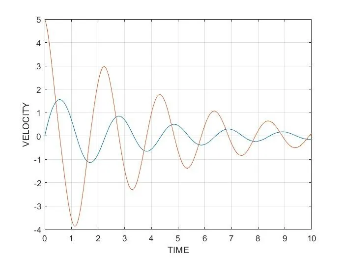
- TO SOLVE THE SECOND ODE WITH GRAPH OF VELOCITY v/s DISPLACEMENT
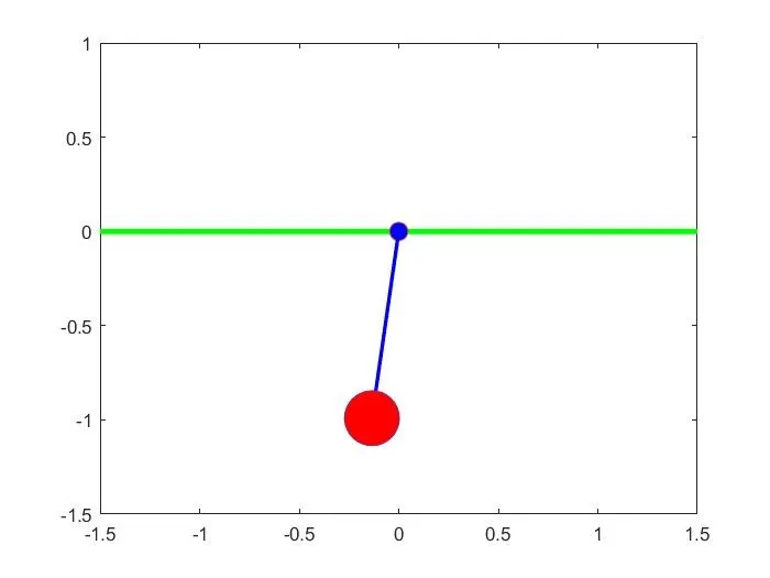
- TO CREATE THE ANIMATION OF THE SIMPLE PENDULUM
PROCEDURE
Damping coefficient (b) = 0.05
gravity (g) = 9.81
length of pendulum (l) = 1
mass (m) =0.1
MATLAB coding:-
Function code
function [dtheta_dt] = ode_func(t,theta,b,g,l,m);
theta1 = theta(1);
theta2 = theta(2);
dtheta1_dt = theta2;
dtheta2_dt = -(b/m)*theta2-(g/l)*sin(theta1);
dtheta_dt =[dtheta1_dt; dtheta2_dt];
end
Main Program Coding
clear all
close all
clc

%program for  ode
b = 0.05;
g = 9.81;
l = 1;
m = 0.1;
%intial condition
theta_0 = [0 5];
%time points
t_span = linspace(0,10,100);

%solve ODE
[t, results]=ode45(@(t,theta) ode_func(t,theta,b,g,l,m),t_span,theta_0);
plot(t, results(:,1))
hold on
plot(t, results(:,2))
ylabel('plot')
xlabel('time')

%for animation
theta3 = results(:,1);
ct = 1;
for i = 1:length(theta3)
T3 = theta3(i)
x0 = 0;
y0 = 0;
x1 = 1*sin(T3);
y1 = -(1*cos(T3));

%for surface line

plot([-5 5],[0 0],'color','g','linewidth',3)
hold on
%for point ocontact of wire and surface
plot([0 0],[0 0],'o','markerfacecolor','b','markersize',10)
hold on
%for wie representation
plot([x0 x1],[y0 y1],'color','b','linewidth',2)

hold on
%for bob representation
plot(x1,y1,'o','markerfacecolor','r','markersize',30)
hold off
axis ([-1.5 1.5 -1.5 1])
pause(0.0002)

 M(ct)= getframe(gcf)
 ct= ct+1;
end
 movie(M)
 Videofile = VideoWriter('secondorder_equation')
 open(Videofile)
 writeVideo(Videofile,M)
 close(Videofile)
CODE EXPLANATION FOR THE ABOVE PROGRAM
1. The First step for the second ODE is we have to derive the main formula
2. By using formulas we can write the entire program.
3. Then used the plot command to plot the graph between the time and velocity, the legend command is sed for the identity of each value in the graph.
4. After getting the plot we need to write a program for the simple pendulum for that we have to write to the program for lines and lengths
5. For getting the simulation of the simple pendulum to the second ODE with damping we need to use the looping statements. the pendulum has fixed coordinates mentioned as x0,y0, and x1,y1 is the other coordinates
6. Marker command is used for making bob of the pendulum, the axis is fixed using axis command. The counter command is used to make the value change in each loop
RESULTS
1. Output for the second ODE for graph for the velocity vs time
2. Animation for the simple pendulum link given below
The link from the google drive and youtube link not working
https://drive.google.com/file/d/1rB3nO3CFmmz-zaLnt_3DIwCp6IRVaHdT/view?usp=sharing
ERRORS
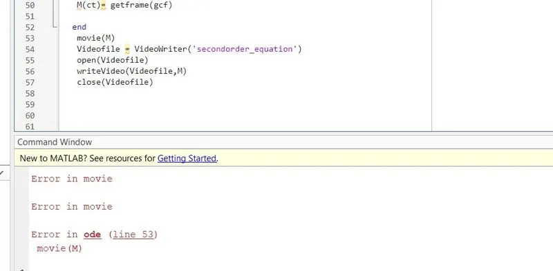
- Errors faced while programming.
while I was writing the program one of the errors that I get mostly I didn't get proper animation until taught by technical expert's suggestion
- How have you overcome those errors.
I just know the function of ct and where should be used
- Screenshots showing errors thrown in command window.