Project 2 - Rankine cycle Simulator
AIM:
- To Create a Rankine Cycle Simulator using OCTAVE/MATLAB
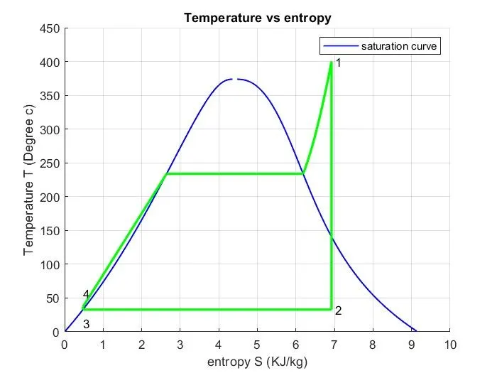
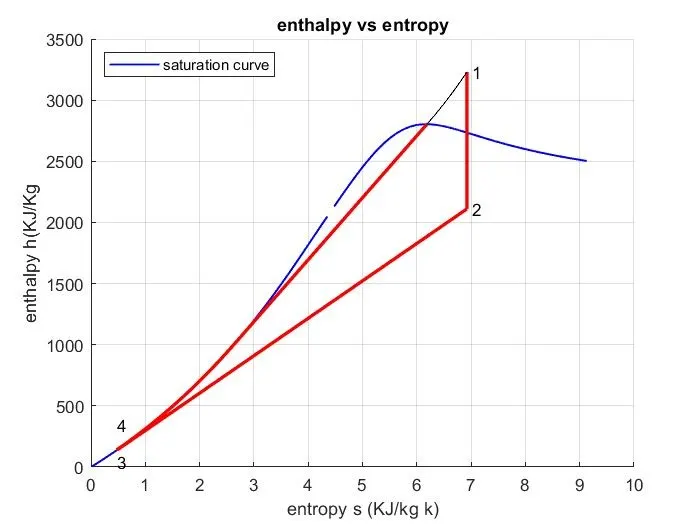
- To plot the corresponding T-s and h-s plots
INTRODUCTION
A Rankine cycle is an idealized thermodynamic cycle or heat engine in which fuel is used to produce heat within a boiler, converting water into steam which then expands through a turbine producing useful work. this process was developed in 1859 by Scottish engineer William j.m Rankine.
It is a cycle that converts heat into mechanical energy which usually is converted into electrical energy.
The process in rankine cyclel are given as:
1. Isentropic compression in pump.
2. constant pressure heat addition in boiler.
3.Isentropic expansion in a turbine.
4.Constant pressure heat rejection in condenser.
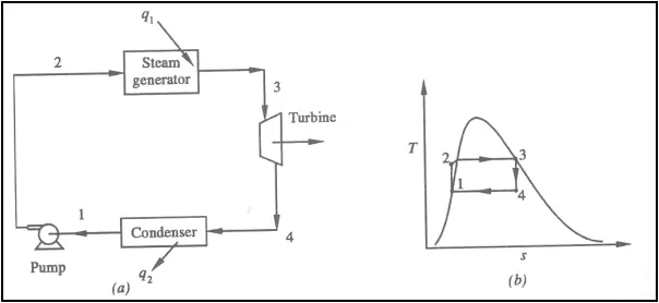
Schematic diagram for rankine cycle:
Procedure for Rankine cycle:
water enters the pump at state as saturated liquid and is compressed isentropically to the operating pressure of the boiler.The water temperature increases some what during this isentropic compression process due to slight decrease in the specific volume of water.The vertical distance between states 1 and 2 on the T-diagram is greatly exaggeratedfor clarity
water enters the boiler as a compressed liquid at state 2and leaves as a superheated vapour at state 3.The boileris bassically a large heat exchanger where the heat originating from combustion gases, nuclear reactors, or other sourcess is transferred to the water essentially at constant pressure.The boiler,together with the section where the steam is superheated(The superheater),is often called the steam generator.
The superheated vapor aat state 3 enters the turbine, where it expands isentropically and procedures work by rotating the shaft connected to an electric generator.The pressureand the temperature of steam drop during this process to the values at state 4, where steam enters the condenser.At this state , steam is usually a staurated liquid-vapor mixture with a high quality. steam condensed at constant pressure in the condenser,which is basically a large heat exchanger, by rejecting heat to a coolong medium such as saturated liquid and enters the pump,completing the cycle. In areas where water is precious, the power plants are cooled by air instead of water.This method of cooling. which is also used in car engines, is called dry cooling
Remembering that the areaunder the process curve on T-s diagram represets the heat transfer forinternally reversible processes, we see that the area under process curve 2-3 represents the heat transferred to the water in the boiler and the area under the process curve 4-1 representsthe heat rejected in the condenser.
All the four components of rankine cycle are steady flow device hence the process regarding this device can be evaluated assteady state process. the steady state flow energy equation per unit mass of steam reduces to
`(qi n - q out) +(Wi n - W out)= he-hi`
Thw boiler and condenser are not involved in any mechanical work where as pump and turbine are assumed to isentropic in nature while working throughout the cycle, then conservation of energy relation for each device can be ecpressed as
`Wpump = h2-h2`
where
h1 = hf at p1 and vf at p1
The work which can be taken out of cycle from turbine is given as
Wout = h3 - h4
the heat removed from the condenser s given as
qin = h3-h2
The heat removed from the condenser is given as
qout = h4-h1
The thermal efficiency of rankine cycle is given as
ηthermal = `(Wn et)/(qi n)`
= `1-(qout)/(qi n)`
Wnet = qin- qout
= Wturb = Wpump
STEP WISE EXPLANATION OF MAIN CODE
1. The creation of rankine cycle simulator starts with some input values which are rquired to calculate the othe state points and used input command
2. The rankine cycle process is displayed in the command window and then inputs are entered inlet pressure for turbine, temperature at turbine inlet and pressure at condenser
3.Then using XSteam function file for reading the state points 1 values
4. As process from 1-2 isentropic compression the entropyy at 1 is qual to point 2
5. The term sg is saturated vapour entropy and sf is saturated liquid entropy
6. Similarly other points takem from XSteam function file.
7.After calculating the net work done, thermal efficiency of rankine cycle is calculated along the specific steam consumption
8.Then the temperature of the each point calculated
9.Then plotting is done respectively for T-s and H-s graph is rankine cycle and each state point values has been shown in command window
Input values :
p1 = 30 bar
T1= 400 degree c
p2 = 0.05 bar
clear all
close all
clc

disp('RANKINE CYCLE')
disp('1-2 isentropic  expansion in the turbine');
disp('2-3 constant pressure heat removal in the condenser');
disp('3-4 isentropic compression in the pump')
disp('4-1 constant pressure heat addition in the boiler');

%obtaining the input data
%p1 -pressure in bar
p1 = input('enter pressure at turbine inlet(in bar)');
T1 = input('entr temperature at turbine inlet (in degree C');
p2 = input('temperrature at condenser inlet in bar');

%state 1

h1 = XSteam ('h_pT', p1, T1); %enthalpy at pressure and temperature 1
s1 = XSteam ('s_pT',p1, T1); %entropy at pressure and temperature 1

%state 2
s2 = s1; % as steam expands isentropically
sf2 = XSteam ('sL_p',p2); % saturated liquid entropy at pressure 2
sg2 = XSteam('sV_p',p2); % saturated vapour entropy at pressure 2
x2 = (s2-sf2)/(sg2-sf2); % fraction at state point 2
hf2= XSteam ('hL_p', p2) % saturated liquid enthalpy at pressure 2
hg2 = XSteam ('hV_p', p2) %saturated vapour enthalpy at pressure 2
h2 = hf2 + (x2*(hg2-hf2)); % enthalpy at state point2

% state 3
p3 = p2   % const pressure heat rejection in condenser
s3 = XSteam('sL_p', p3); %saturated liquid entropy at pressure 3
h3 = XSteam('hl_p', p3); %saturated liquid enthalpy at pressure 3

% sttae 4
p4= p1; %constant pressure heat rejection
s4 = s3; %isentropic compression process

% work done by pump
v3 = XSteam('vL_p', p3);
Wp = v3*(p4 - p3)*100; % work done for pump
h4 = h3 + Wp; %enthalpy at state point 4

% work done by the turbine

Wt = h1 - h2;

% net work
Wnet = Wt - Wp;

% heat in of the system
Qin= h1-h4;

% heat out of the system
Qout = h2 -h3;

% Thermal efficiency
efficiency = (Wnet/Qin)*100;

%specific steam consumption
SSC = (3600/Wnet);

% calculating temperature at the state points
T3 = XSteam ('Tsat_p', p3);%saturation temperature at pressure 3
T2 = T3; %constant pressure heat addition
Cp4 = XSteam('Cp_ps', p4, s4); %specific constant pressure heat capacity
Cv4 = XSteam('Cv_ps', p4, s4); %specific constant volume heat capacity
k = Cp4/Cv4;
T4 = T3/((p3/p4)^((k-1)/k)); %temperature at state point 4

% Calculating temperature, entropy, and enthalpy at the Vapour and liquid
% line for plotting

T6 = XSteam('Tsat_p', p1); %saturated temperature at pressure 1
s5 = XSteam('sL_p',p1); %saturated Liquid entropy at pressure 1
s6 = XSteam('sV_p', p1); %saturated vapour entropy at pressure 1
h5 = XSteam('hL_p', p1); %saturated Liquid enthalpy at pressure 1
h6 = XSteam('hV_p',p1); %saturated vapour enthalpy at pressure 1
T5 = T6;

%plotting the saturation curve
T = linspace(1,375,1000);
for i = 1:length(T)
    sf(i) = XSteam ('sL_T', T(i)); %saturated Liquid entropy
    sg(i) = XSteam ('sV_T', T(i)); %saturated vapour entropy
    hf(i) = XSteam('hL_T', T(i)); %saturated Liquid enthalpy
    hg(i) = XSteam ('hV_T', T(i)); %saturated vapour enthalpy

end

% plotting T-s diagram
figure(1)
hold on
plot(sf, T, 'r','linewidth',1,'Color','b')
plot(sg,T,'r','linewidth',1,'Color','b')
plot([s1 s2],[T1 T2], 'k', 'linewidth',2,'Color','g')
plot([s2 s3], [T2 T3],'k','linewidth',2,'Color','g')
plot([s3 s4], [T3 T4],'k','linewidth',2,'Color','g')
plot([s4 s5], [T4 T5], 'k', 'linewidth',2,'Color','g')
plot([s5 s6],[T5 T6],'k','linewidth',2,'Color','g')
sc1 = linspace(s6, s1,2000);
for l = 1:length(sc1);
    Tc1(l) =XSteam('T_ps', p1,sc1(l))
end
plot(sc1,Tc1, 'k','linewidth',2,'Color','g')
text(s1+0.1,T1, '1')
text(s2+0.1,T2, '2')
text(s3,T3-20, '3')
text(s4,T4+20, '4')
title('Temperature vs entropy')
xlabel ('entropy S (KJ/kg)')
ylabel ('Temperature T (Degree c)')
legend('saturation curve')
grid on


%plotting h-s Diagram
figure(2)
hold on
plot(sf,hf,'r','linewidth',1,'Color','b')
plot(sg,hg,'r','linewidth',1,'Color','b')
plot([s1 s2],[h1 h2],'k','linewidth',2,'Color','r')
plot([s2 s3],[h2 h3],'k','linewidth',2,'Color','r')
plot([s3 s4],[h3 h4],'k','linewidth',2,'Color','r')
hc = linspace(h4,h5,1000);
for k = 1:length(hc)
    sch(k) = XSteam('s_ph', p1, hc(k))
end
plot(sch,hc,'k','linewidth',2,'Color','r')
plot([s5 s6],[h5 h6], 'k','linewidth',2,'Color','r')
for m = 1:length(sc1)
    hc1(m) = XSteam('h_ps',p1,sc1(m))
end
plot(sc1, hc1, 'k')
text(s1+0.1,h1,'1')
text(s2+0.1,h2,'2')
text(s3,h3-100,'3')
text(s4,h4+200,'4')
title('enthalpy vs entropy')
xlabel ('entropy s (KJ/kg k)')
ylabel ('enthalpy h(KJ/Kg')
legend('saturation curve','location', 'northwest')
grid on

% Displaying Results
disp('RESULTS')
fprintf('At state point 1:n')
fprintf('p1: %8.3f barn', p1)
fprintf('T1 : %8.3f Cn',T1)
fprintf('h1:%8.3f KJ/kgn', h1)
fprintf('s1 : %8.3f KJ/kgknn',s1)

fprintf('At state point 2:n')
fprintf('p2: %8.3f barn', p2)
fprintf('T2 : %8.3f Cn',T2)
fprintf('h2:%8.3f KJ/kgn', h2)
fprintf('s2 : %8.3f KJ/kgknn',s2)
fprintf('x2: %8.3fnn', x2)

fprintf('At state point 3:n')
fprintf('p3: %8.3f barn', p3)
fprintf('T3 : %8.3f Cn',T3)
fprintf('h3:%8.3f KJ/kgn', h3)
fprintf('s3 : %8.3f KJ/kgknn',s3)

fprintf('At state point 4:n')
fprintf('p4: %8.3f barn', p4)
fprintf('T4 : %8.3f Cn',T4)
fprintf('h4:%8.3f KJ/kgn', h4)
fprintf('s4 : %8.3f KJ/kgknn',s4)

fprintf('Turbine Work: %8,3f KJ/kgn', Wt)
fprintf('Pump Work: %8.3f KJ/kgn',Wp)
fprintf('Wnet: %8.3f KJ/kgn', Wnet)
fprintf('Efficiency: %8.3f Percent n ', efficiency)
fprintf('S.S.C: %8.3f KJ/kWh',SSC)
RESULTS : finally created the rankine cycle simulator for thee given input. output plots for the rankine cycle are shown below
RESULTS IN COMMAND WINDOW
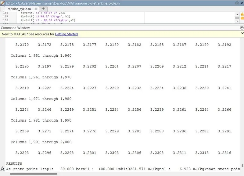
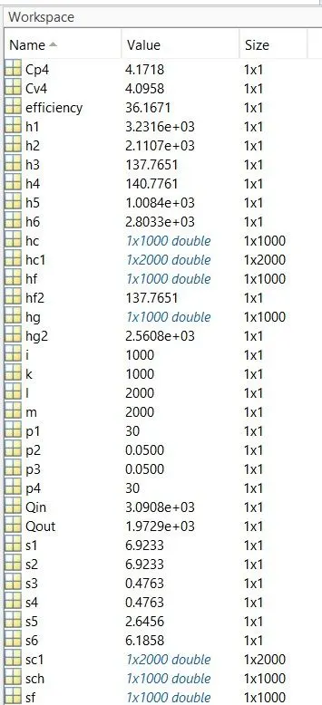
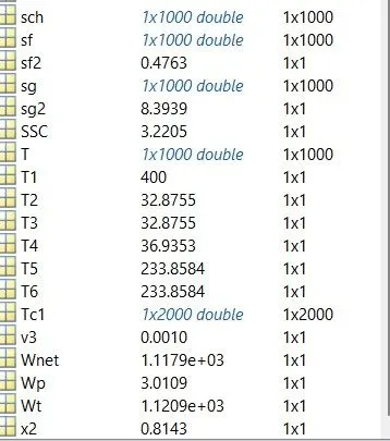
RESULTS IN COMMAND WORKSPACE
ERRORS
- Mention the errors faced while programming.
Mostly errors that i faced were wrote the formulas wrong & forget to write the k & T values .
- Steps taken to overcome those errors.
By help of error showing in the command window chceking the entire formulas and rectify the problem and rn the entire coding.
REFERANCES:http://home.iitk.ac.in/~suller/lectures/lec29.htm
https://universe.bits-pilani.ac.in/uploads/VAPUR%20POWER%20CYCLE.pdf
THERMODYNAMICS TEXT BOOK