Simple Pendulum Animation using MATLAB.

Creating a Simple Pendulum by solving Second-Order ODEs.

AIM:

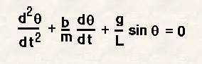
• Write a program to solve the above ODE and a program that will simulate the pendulum motion.
• To create a plot between angular velocity and displacement of the simple pendulum by using ode45.
• To create an animation of a simple pendulum by using the ODE solver program that we are going to write.

CONCEPT:

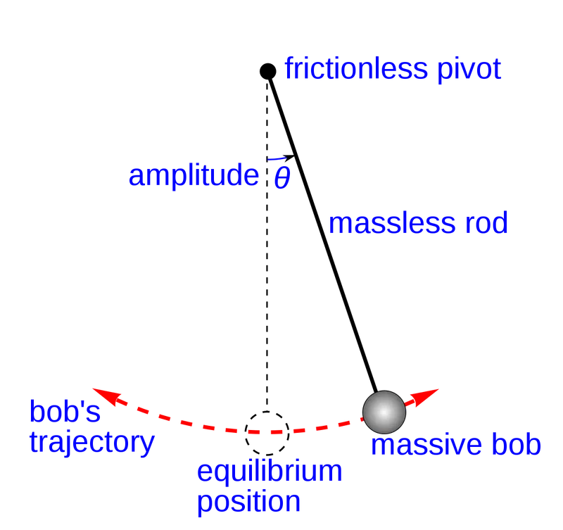
A simple pendulum is a mechanical arrangement that demonstrates periodic motion. The simple pendulum comprises a small bob of mass ‘m’ suspended by a thin string secured to a platform at its upper end of length L. The simple pendulum is a mechanical system that sways or moves in an oscillatory motion. This motion occurs in a vertical plane and is mainly driven by the gravitational force.

From the above equation of a simple pendulum with a damping factor, we know

b = damping coefficient (N-m/s)

m = mass of the bob (kg)

g = gravitational acceleration (m/s)

l = length of the string to connect the bob (m)

As we can see the above equation have a differential power order of 2. We have to solve this 2nd order differential equation into a simple differential equation in order to use the ode45 solver in Matlab.

Simplifying the above 2nd order equation.

Now let us consider,

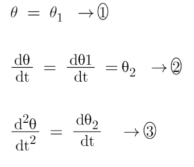
Substituting the Eq 1,2,3 values into the 2nd order equation the equation becomes;

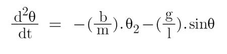
Now we will simplify the differential equation into the form of a matrix,

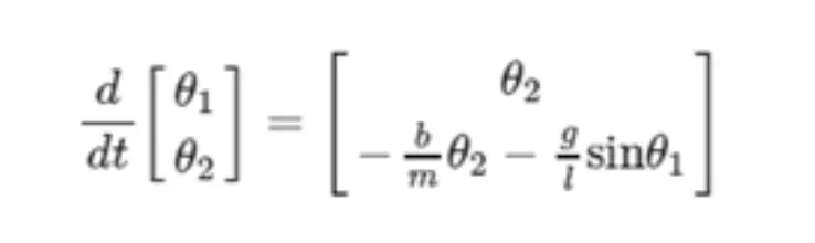
Now that we have the required equation we can solve this in Matlab using the ode45 solver and plot the required Graph and make an animation of the simple pendulum.

Staring with the ODE function Program:

function [dtheta_dt] = challenge_ode_func(t,theta,b,g,l,m)
theta1 = theta(1);
theta2 = theta(2);
dtheta1_dt = theta(2);
dtheta2_dt = -(b/m)*theta2 - (g/l)*sin(theta1);
dtheta_dt = [dtheta1_dt; dtheta2_dt];
end

Program Explanation:

• So in the above code, I have created a function named "challenge_ode_function" which has the ability to take input values and assign value to the output array.
• Then I wrote down the value of "theta1" and "theta2".
• Then in the next steps, I wrote the values for "dtheat1_dt" and "dtheta2_dt".
• In the final step, I wrote down the dtheta_dt into a column matrix which included the values "dtheta1_dt and dtheat2_dt" and used the end command to stop the function.

Now for the program of the simple pendulum.

% Program for Simple Pendulum
clear all
close all
clc

% Input Variables reuired for solving the 2nd order ODE equation
b = 0.05;
g = 9.81;
l = 1;
m = 0.1;

theta_0 = [0; 3];

t_span = linspace(0,20,500);

% ode45 Function to solve second order ODE
[t,results] = ode45(@(t,theta) challenge_ode_func(t,theta,b,g,l,m),t_span, theta_0);

% Plotting of Angular Velocity and Displacement
figure(1)
plot(t,results(:,1))
hold on
plot(t,results(:,2))
grid on
title('Motion of Pendulum')
xlabel('Time in Sec')
ylabel('Angular Velocity(rad/s) and Displacement(rad)')
legend('Displacement','Angular Velocity')

angle = results(:,1);

% Counter Command for iterations.
ct = 1;

for i = 1 : length(angle)
    omega = angle(i);
    figure(2)
    title('Motion of Pendulum')
    
    % Fixed Coordinates of one end of the simple pendulum.
    x0 = 0;
    y0 = 0;
    
    % Moving Coordinates of the bob.
    x1 = l*cos((3*pi/2)+omega);
    y1 = l*sin((3*pi/2)+omega);
    
    % Plotting of the Bob Motion
    plot([x0 x1],[y0 y1],'linewidth',3,'color','y');
    hold on;
    plot(x1,y1,'o','markers',15,'MarkerFaceColor','r');
    hold on;
    plot([-3 3],[0,0],'linewidth',5,'color','b');
    hold off
    axis([-3 3 -2 2])
    grid on
    title('Animation of Simple Pendulum')
    pause(0.1)
    M(ct) = getframe(gcf);
    ct = ct+1;
end

% To create a Animation of the Simple Pendumlum
movie(M)
videofile = VideoWriter('simple_pendulum.avi','Uncompressed AVI');
open(videofile)
writeVideo(videofile,M)
close(videofile)

Program Explanation:

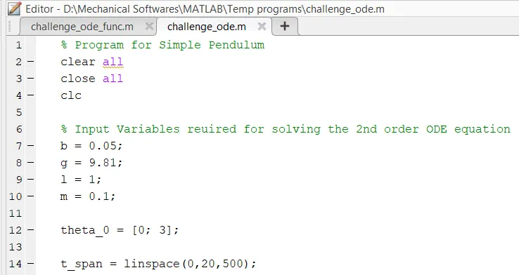
• clear all, close all, clc are used to clear the workspace, clear any graphs and clear the command window.
• Now in the next part, I mentioned the input values required for the solving of the equation, where: b = damping coefficient = 0.05 (n-m/s), g = acceleration due to gravity = 9.81 (m/s), l = length of string = 1 (m), m = mass of the bob = 1 (kg).
• t_span is a command used in the ode45 solver which specifies the time span of the iterations that are going to solve the ordinary differential equation. As we needed an array of values I also used the linspace command.

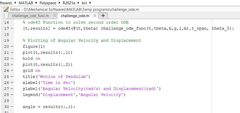
• ode45 is a function in Matlab that solves ordinary or partial differential equations using a numerical method. In this problem, the highest order is 2 so I took two constant values so that the equation is changed to the simple differential equation. The function should have at least 2 inputs to solve the equation to the approximate result.
• The ode45 function has a syntax in which we need to specify which should be 't' and 'y' and the output may be of (t, y, args) and a timespan for the function to work and the initial value of the equation.
• Syntax of an ode45 solver is as follow:

[t,results] = ode45(@(t,y)ode(t,y,args),t_span,y0);

• Now for the plotting purpose let's start with figure 1 this will tell us how the damping is done for the pendulum. The angular velocity and displacement will come to rest at end of the function.
• Plotting the values of the angular velocity and the displacement by using the plot command.
• Using the label command to label the x and y-axis and the title command to give the title to the graph.
• legend command is used to label the angular velocity and the displacement.

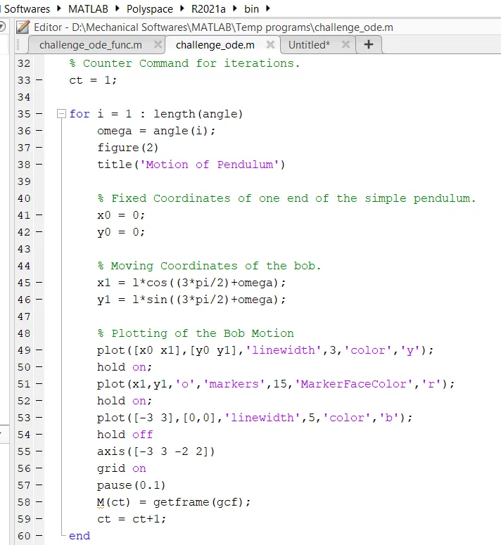
• Now toward the part of creating the simple pendulum animation, I started off with a counter command a gave it the value 1 so that I can use the for loop command to create the specified set of points to keep the bob at different locations.
• In the for loop, I defined the variable "i" as 1 is to length in terms of the angle. Also assigned omega as angle(i).
• Then I defined the x0 and y0 points as fixed points of the string and x1 and y1 will be the different positions of the bob.
• Now for plotting the bob motion, we used the plot command to plot the pendulum rod first, followed by the fixed point and the bob.
• I gave the plotting specific points so that the animation will be in the center, also included the pause command to pause the frames at a certain interval.
• At the end combine all the collected frames and create an animation out of it using the M(ct) command so that all collected frames will be converted into a single output.

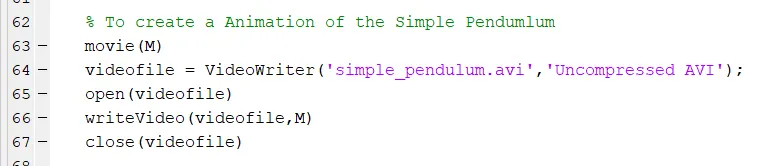
• Toward the last part of the code and creation of an avi file of animation, used the movie(M) command to create a movie of the animation.
• videofile and videoWriter command for giving the name of the video file and its format.
• open command to open that videofile.
• writeVideo command to write the collected frames into the videofile.
• Finally, the close command to close the videofile.

Errors:

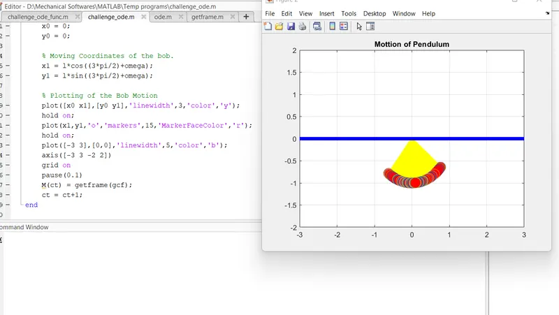
• I was getting my animation like this at first because I didn't include the hold off command, I was not aware of this so did some research, and then when I included hold off command the problem was cleared.

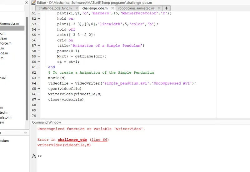
• This was the other error I was facing this was a simple typo as I accidentally wrote writeVideo command as writerVideo.

Outputs:

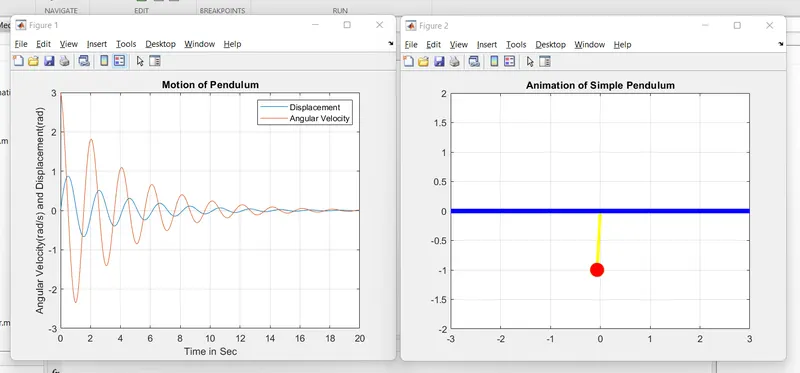
• Figure one shows the plot between the angular acceleration and displacement of the motion of the simple pendulum.
• The blue curve is the displacement that starts from zero and the red curve is the angular velocity which starts from 3 (rad/sec).
• At the end of the t_span, both the displacement and angular velocity becomes zero and the motion of the simple pendulum becomes zero which becomes rest.
• Figure two is the animation plot of the simple pendulum I am attaching the video file of the animation below.
• Animation of the Simple Pendulum: https://drive.google.com/file/d/1IozI2lvaByL4riRVem2Phhzqr3P2gm46/view?usp=sharing

Conclusion:

• We have animated the simple pendulum using the ode45 solver where the second-order is reduced to a simple differential equation where it is easy to solve the given equation.
• The animation is created using the different points of the bob and the motion of the simple pendulum.