Curve Fitting using MATLAB.

AIM: To write a code to perform curve fitting in MATLAB.

OBJECTIVES:

1. Write a code to fit a linear and cubic polynomial for the Cp data provided.
2. Plot the linear and cubic fit curves along with the raw data points.
3. Write a code to show the splitwise method.
4. Explain the parameters used to measure the fitness characteristics for both curves.

THEORY:

Curve fitting is the process of constructing a curve, or mathematical functions, which possess the closest proximity to the real series of data. By curve fitting, we can mathematically construct the functional relationship between the observed dataset and parameter values, etc. It is highly effective in the mathematical modeling of some natural processes.

The curve fit is important to know the trend followed by data and also allow additional mathematical operation which might not be possible in the initial data set. For example, the population data in-country. There is no formula to find what the population is going to be in next year. However, if we fit a curve, we had a function that says how the population is going to change with respect to time. The accuracy of results depends on the quality of curve fit but at least we can have a rough trend.

Choosing the best fit depends upon finding a curve that satisfies the data points there are 4 quantities that help us measure the goodness of fit criteria or how well the equation is representing the data points. They are:

1. The sum of squares due to error (SSE).
2. R-square.
3. Adjusted R-square.
4. Root mean squared error (RMSE).

1. The sum of squares due to error (SSE)

Assume data points (x1,y1), (x2,y2), (x3,y3),....(xn,yn) and assume the best fit for these set of points will be y = f(X), the criterion under which the equation of the curve will be the best fit possible is as follows,

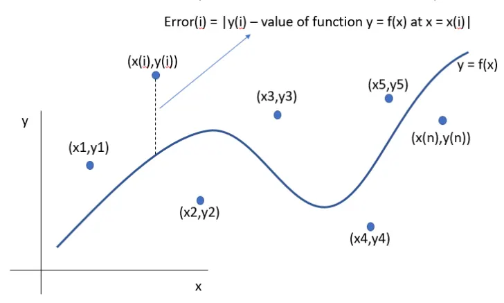
Suppose each of these n points has an individual error (difference in y co-ordinate values)

The error for a general T point can be given by the function,

To remove the modulus sign, it is effective if we square the error term, when we square the error terms and add the errors for all the 'n' points we get,

Assume the proposed equation is a nth degree polynomial of the form,

When we differentiate the SSE with each and every coefficient of the proposed equation f(x) and equate it to zero, we can find the minima and the value of that coefficient.

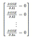
Upon solving the multiple systems of equations we can find the values of all the coefficients.

This method is known as the Least Squares Method and is the most commonly used technique as long as the fitting function is a polynomial.

2. R-square.

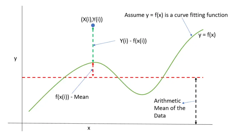
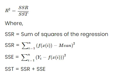
This quantity measures how successful the fit is in explaining the variation of the data. Put another way, R-square is the square of the correlation between the response values and the predicted response values. It is also called the square of the multiple correlation coefficient and the coefficient of multiple determination.

That is the higher the value of R-square the better the fit, the lower it is the lousier the fit, R-square ranges from a value of 0 to 1 0

• 0 for the worst possible fit for the data set.
• 1 for the best possible fit for the data set.

3. Adjusted R-square.

Adjusted R-square is a normalizing variation of R-square which neglects the variation of R-square due to insignificant independent variables.

• If the value of x(i) contributes to the output y, then x(i) is a significant dependent variable.
• If the value of x(i) does not contribute to the output y, then x(i) is an insignificant dependent variable.

Adjusted R-square disregards these infinitesimally small increments to R-square, and only considers the variables which actually contribute to the output of the system in a drastic way.

R-square is formulated as below,

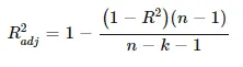
Where,

n = the number of data points.

k = the number of independent variables.

Here, there can be 2 possibilities:

1. The newly added independent variable is significant.
2. The newly added independent variable is insignificant.

4. Root mean squared error (RMSE).

This statistic is also known as the fit standard error and the standard error of the regression. It is an estimate of the standard deviation of the random component in the data, and is defined as,

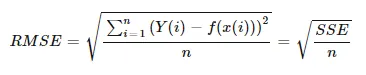
where n is the total number of data points available.

Using these four quantities Matlab effectively deduces the goodness of fit, typically if R-square is greater than 0.95 the fit is assumed to be good.

PROGRAM:

clear all
close all
clc

% Loading the data file which has values of Cp at various temperature
cp_data = load('data');
temperature = cp_data(:,1);
cp = cp_data(:,2);

% Curve Fitting
% For linear function which has a polynomial degree of 1 | Cp = a*t+b
co_effs1 = polyfit(temperature,cp,1);
predicted_cp1 = polyval(co_effs1,temperature);

% For cubic function which has a polynomial degree of 3 | Cp = a*t^3+b*t^2+ct+d
co_effs2 = polyfit(temperature,cp,3);
predicted_cp2 = polyval(co_effs2,temperature);

% Lets compare the original plot with linear curve fit
figure(1)
subplot(2,1,1)
% Plotting the original plot
hold on
plot(temperature,cp,'linewidth',3);
% Plotting the linear curve fit
plot(temperature,predicted_cp1,'linewidth',3,'color','r');
xlabel('Temperature [K]');
ylabel('Specific Heat (Cp) [KJ/Kmol-k]');
legend('Original Data Set','Linear Curve Fit');
title('Linear Curve Fit');
hold off

% Now lets compare the original plot with our cubic curve fit
subplot(2,1,2)
% Plotting the original plot
hold on
plot(temperature,cp,'linewidth',3);
% Plotting of the cubic curve fit
plot(temperature,predicted_cp2,'linewidth',3,'color','c');
xlabel('Temperature [K]');
ylabel('Specific Heat (Cp) [KJ/Kmol-k]');
legend('Original Data Set','Cubic Curve Fit');
title('Cubic Curve Fit');
hold off

% Now lets compare all the plots (original plot, Linear Fit and Cubic fit)
figure(2)
hold on
plot(temperature,cp,'linewidth',2);
plot(temperature,predicted_cp1,'linewidth',3,'color','r');
plot(temperature,predicted_cp2,'linewidth',3,'color','c');
xlabel('Temperature [K]');
ylabel('Specific Heat (Cp) [KJ/Kmol-k]');
legend('Original Data Set','Linear Curve Fit','Cubic Curve Fit');
title('Linear vs Cubic Fit');
hold off

% Calculation for the best fit.
% Calculation of Sum of Squares due to Error (SSE)
SSE_L = sum((cp-predicted_cp1).^2);     % For Linear Fit
SSE_C = sum((cp-predicted_cp2).^2);     % For cubic Fit

% Calculation of R-square
M = mean(cp);           % Mean for the R-square Calculation
% For Linear Fit
SSE_linear = sum((cp - predicted_cp1).^2);      % Sum of squared errors
SSR_linear = sum((predicted_cp1 - M).^2);       % Sum of squares of regression

SST_linear = SSE_linear+SSR_linear;             % Total of sum of squares

% Calculating R-square for Linear fit
Rsquare_L = SSR_linear/SST_linear;

% For Cubic Fit
SSE_cubic = sum((cp - predicted_cp2).^2);      % Sum of squared errors
SSR_cubic = sum((predicted_cp2 - M).^2);       % Sum of squares of regression

SST_cubic = SSE_cubic+SSR_cubic;             % Total of sum of squares

% Calculating R-square for Cubic fit
Rsquare_C = SSR_cubic/SST_cubic;

% Calculation of Adjusted R-square
k = 1;
AdRsquare_L = 1- (((1-Rsquare_L)*(length(cp)-1))/(length(cp)-k-1));      % For Linear Fit
AdRsquare_C = 1- (((1-Rsquare_C)*(length(cp)-1))/(length(cp)-k-1));      % For Cubic Fit

% Calculation of Root Mean Squared Error (RMSE)
RMSE_L = sqrt(SSE_L/length(cp));        % For Linear Fit
RMSE_C = sqrt(SSE_C/length(cp));        % For Cubic Fit

% Putting Errors in form of a Table
Name_of_Errors = {'SSE';'R_Square';'AdjustedR_Square';'RMSE'};

Linear_Fit_Error = [SSE_L; Rsquare_L; AdRsquare_L; RMSE_L];
Cubic_Fit_Error = [SSE_C; Rsquare_C; AdRsquare_C; RMSE_C];

disp('BestFit Parameter for Linear and Cubic Curve Fit')
BestFit_Parameters = table(Linear_Fit_Error,Cubic_Fit_Error,'RowNames',Name_of_Errors);

EXPLANATION OF CODE:

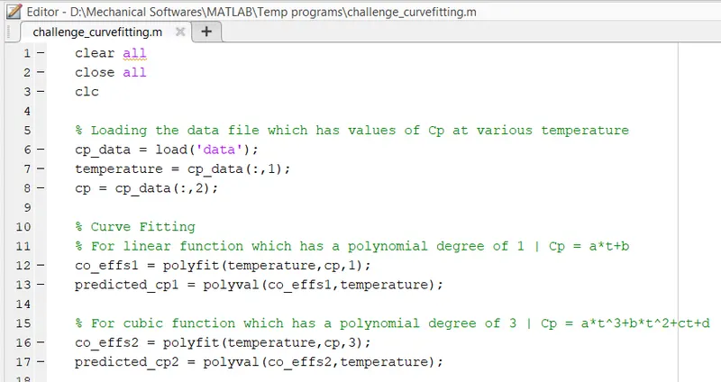
• Starting of the command with the clear all close all and clc command.
• Then I wrote the code to import the data file and gave it the name cp_data. The assigned the 1st column as the temperature and 2nd column as the cp for the certain temperature value.
• For the curve fitting process in the linear function and cubic function with degrees 1 & 3 respectively I used the ployfit and polyval command for the purpose of curve fitting. The polyfit command returns the coefficient in the equation considering the equation y = Ax^2+Bx+C, here the coefficients A, B, and C are calculated.
• The linear function where Cp =a*t+b the ployfit command is used to find the values of the coefficient a and b and the polyval command is used to calculate the predicted values of Cp using the linear equation.
• The cubic function where Cp = a*t^3+b*t^2+ct+d the ployfit command is used to find the values of the coefficient a,b,c, and d, and the polyval command is used to calculate the predicted values of Cp using the cubic equation.

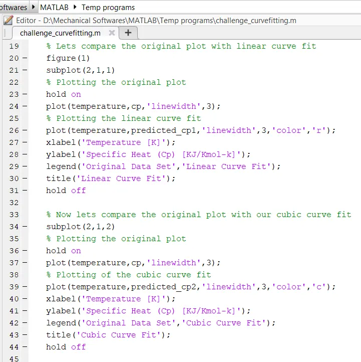
• The first plot command is for the plotting of the linear fit curve vs the original plot and the 2nd plot command is for the plotting of the cubic fit curve vs the original plot.
• Now towards the plotting part, I used the subplot command so that both the linear and cubic curves will be in one single figure and this will be easy to compare.
• Other commands used are plot for plotting purposes, linewidth to give width to the line, xlabel and ylabel for the labeling of x and y-axis, and the legend and title command for the details of the plot also the hold on and hold off commands where used in the start and end.

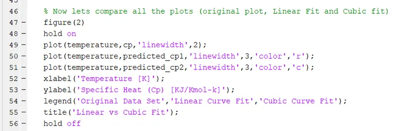
• In this part, I wrote the command for the plotting of all three curves the original plot, the linear fit curve, and the cubic fit curve into a new figure (2).

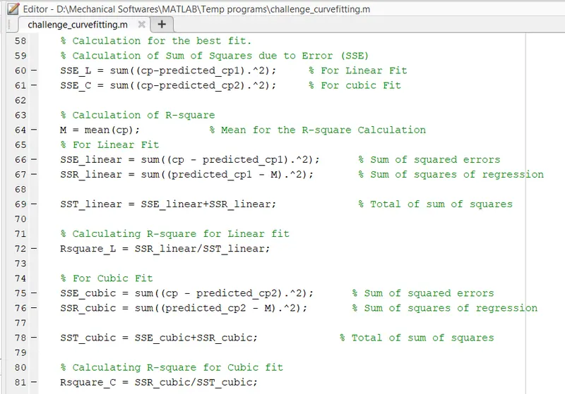
• Now towards the part of the calculation for the best fit curve.
• Starting off with the Sum of Squares due to Error (SSE) method wrote down the formula required to solve for the linear fit as SSE_L and cubic fit as SSE_C.
• Now to the next method i.e. the R-square method, we require the value of mean for the calculation so I wrote the M mean formula. Then for the linear fit, the Sum of squared errors formula is given by SSE_linear, and the Sum of Squares of regression is given by SSR_linear. The total sum of the squares is given by SST_linear, for the calculation of the R-square for the linear fit its formula is given by Rsquare_L.
• Similarly for the cubic fir part, the Sum of squared errors formula is given by SSE_cubic, and the Sum of Squares of regression is given by SSR_cubic. The total sum of the squares is given by SST_cubic, for the calculation of the R-square for the cubic fit its formula is given by Rsquare_C.

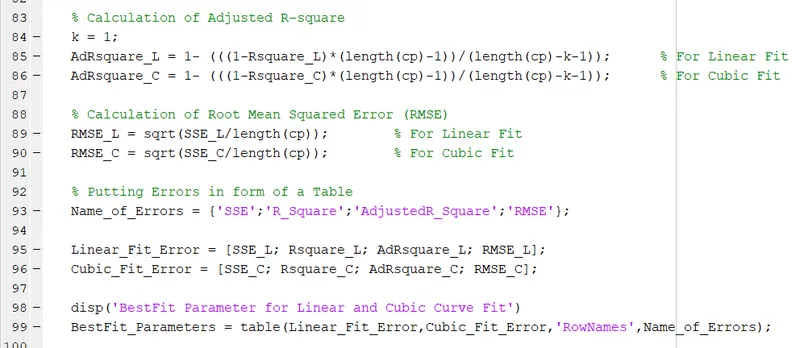
• Now for the Calculation of best-fit curves using the Adjusted R-square method k is the number of independent variables.
• The formula for Adjusted R-square for linear is given by AdRsquare_L and for the cubic is given by AdRsquare_C.
• And to the last method i.e. Root Mean Squared Error (RMSE) the formula for the linear fit is given by RMSE_L and for cubic is given by RMSE_C.
• Now toward the final part of programming, I made a table to store the values in tabular form that are been calculated I used the table command for the making of the table.

RESULTS:

1. This plot shows the comparison of the Linear fit with the original plot and also shows the comparison of Cubic fit with the original plot.

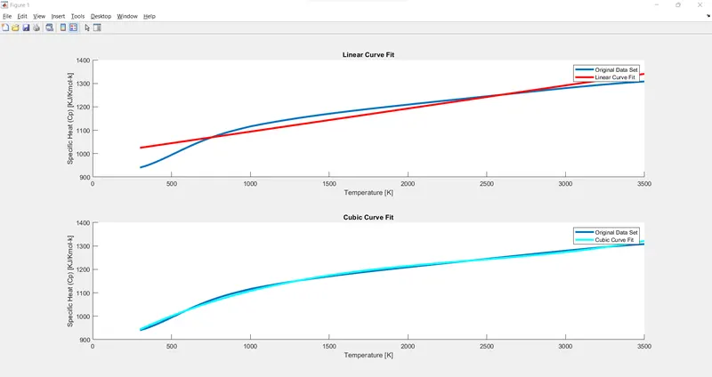
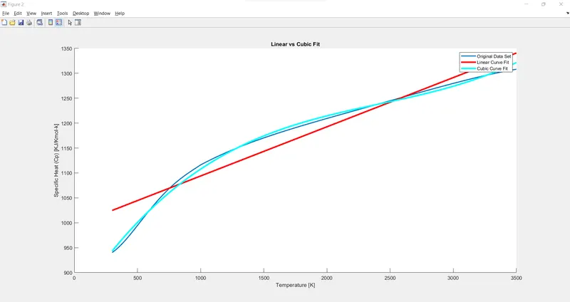
2. This Plot shows the direct comparison between the Linear fit, the Cubic fit, and the Original plot.

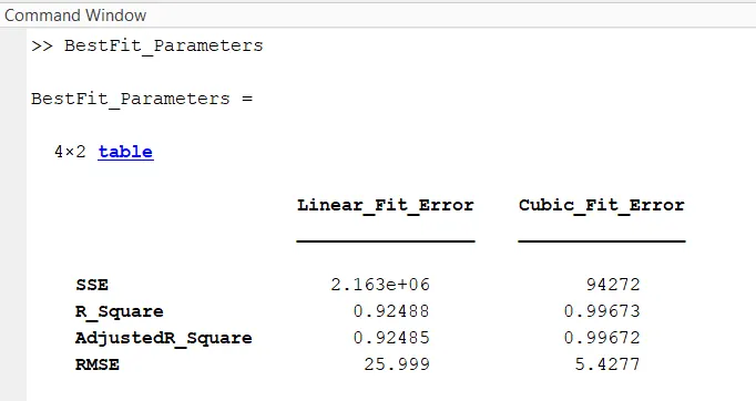
3. This is the output in the command window, which shows the Best fit factor for each curve in a tabular form.

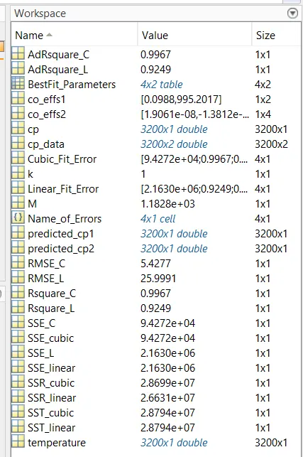
4. These are variables stored in the workspace after running the program.

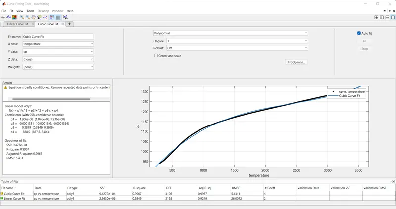
5. And Finally the output using the curve fitting toolbox in MATLAB to validate our fitness characteristics.

5.1. For Linear Fit Curve.

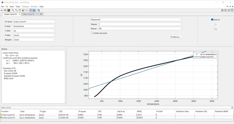
5.2. For Cubic Fit Curve.

PROGRAM:

For Splitwise fitting of Cubic Function:

clear all
close all
clc

% Loading the data file which has values of Cp at various temperature
cp_data = load('data');
temperature = cp_data(:,1);
cp = cp_data(:,2);

% Dividing Temperature and Specific Heat into 5 parts
temperature_1 = cp_data(1:640,1);
predicted_cp_1 = cp_data(1:640,2);

temperature_2 = cp_data(641:1280,1);
predicted_cp_2 = cp_data(641:1280,2);

temperature_3 = cp_data(1281:1920,1);
predicted_cp_3 = cp_data(1281:1920,2);

temperature_4 = cp_data(1921:2560,1);
predicted_cp_4 = cp_data(1921:2560,2);

temperature_5 = cp_data(2561:3200,1);
predicted_cp_5 = cp_data(2561:3200,2);

% For Linear Polynomial | Cp = a*t+b
[co_efficient_lp, s1,mu1] = polyfit(temperature_1,predicted_cp_1,3);
predicted_specific_heat_1 = polyval(co_efficient_lp,temperature_1, s1,mu1);

% For Quadratic Polynomial | Cp = a(t^2)+b(t)+c
[co_efficient_Qp, s2,mu2] = polyfit(temperature_2,predicted_cp_2,3);
predicted_specific_heat_2 = polyval(co_efficient_Qp,temperature_2, s2,mu2);

% For 3rd Degree Polynomial | Cp = a(t^3)+b(t^2)+c(t)+d
[co_efficient_3p, s3,mu3] = polyfit(temperature_3,predicted_cp_3,3);
predicted_specific_heat_3 = polyval(co_efficient_3p,temperature_3, s3,mu3);

% For 4th Degree Polynomial | Cp = a(t^4)+b(t^3)+c(t^2)+d(t)+e
[co_efficient_4p, s4,mu4] = polyfit(temperature_4,predicted_cp_4,3);
predicted_specific_heat_4 = polyval(co_efficient_4p,temperature_4,s4, mu4);

% For 5th Degree Polynomial | Cp = a(t^5)+b(t^4)+c(t^3)+d(t^2)+e(t)+f
[co_efficient_5p, s5,mu5] = polyfit(temperature_5,predicted_cp_5,3);
predicted_specific_heat_5 = polyval(co_efficient_5p,temperature_5,s5, mu5);

% Curve Fit Plot
figure(1)
plot(temperature,cp,'linewidth',2)
hold on
plot(temperature_1,predicted_specific_heat_1,'color','m','linewidth',3)
plot(temperature_2,predicted_specific_heat_2,'color','y','linewidth',3)
plot(temperature_3,predicted_specific_heat_3,'color','b','linewidth',3)
plot(temperature_4,predicted_specific_heat_4,'color','g','linewidth',3)
plot(temperature_5,predicted_specific_heat_5,'color','r','linewidth',3)
hold off
xlabel('Temperature [K]')
ylabel('Specific Heat [KJ/Kmol-K]')
title('Split Wise Curve Vs Original Curve Fit')
axis([250 3600 900 1400])
legend('Original Data','Linear Curve','Quadratic Curve','4th Degree Curve','5th Degree Curve','location','best')

EXPLANATION OF CODE:

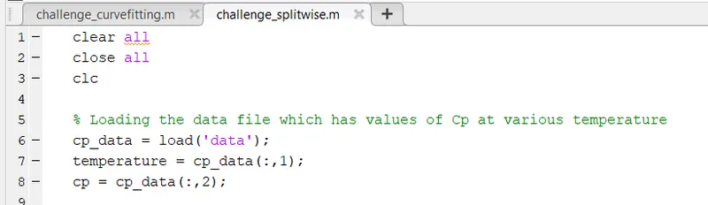
• Starting off with the clear all close all and clc commands.
• Then wrote the code to upload the data file of the Values of Cp at Various Temperatures.

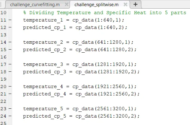
• Now, I have decided to divide the Temperature and Specific Heat into 5 Parts starting from 1 to 3200. These will be defined as temperature_(n) and predicted_cp_(n).

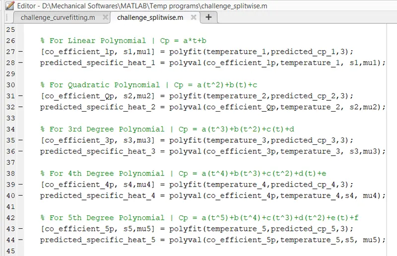
• For the stepwise procedure, we will start off with the Linear Polynomial which is given by Cp = a*t+b, then the Quadratic Polynomial which is given by Cp = a(t^2)+b(t)+c, then comes the 3rd Dregree Polynomial which is given by Cp = a(t^3)+b(t^2)+c(t)+d, then the 4th Degree Polynomial which is given by Cp = a(t^4)+b(t^3)+c(t^2)+d(t)+e and lastly the 5th Degree Polynomial which is given by Cp = a(t^5)+b(t^4)+c(t^3)+d(t^2)+e(t)+f
• These all are written in the required formatting code for easy plotting purposes.

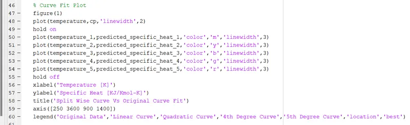
• And lastly, the Plotting of the Stepwise Fit Curve, I used here various different color commands to indicate the different lines, also used the xlabel and ylabel and title to add details to the plot and the legend command for the identification of the curves.

RESULTS OF STEPWISE:

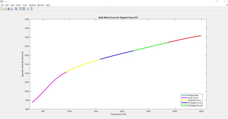
This is the plot of Stepwise VS Original Curve Fit it has every single curve the original, the linear, the quadratic, the 4th degree and the 5th degree one.

ERRORS:

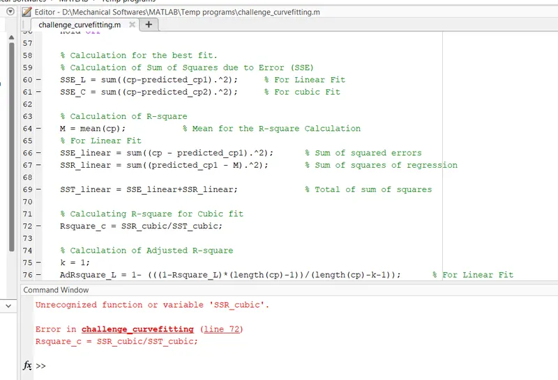
This was the 1st Error I got actually I missed some steps and then for the calculation of R-square Cubic Fit which led me to the error I fixed the code entered all the required values and inputs and formula the error got removed and the code was successful.

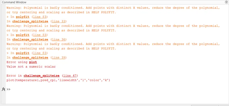
This was the error I was facing while the coding of the stepwise plotting there were many errors when I tried for the 1st time, I then did some research then I got a clear idea of how to code for the Splitwise method.

CONCLUSiON:

1. The linear and polynomial curves are fitted to specific heat data provided using MATLAB.

2. BestFit parameters for each curve are evaluated and are compared with the results using the MATLAB toolbox.

3. The Cubic curve fit is a good fit than the linear curve fit, and this is verified by the BestFit parameters calculated as we can see the R-square value for the Linear fit is 0.92488 and for Cubic fit is 0.99673 which is more close to 1.

REFERENCES:

1. https://in.mathworks.com/help/curvefit/curve-fitting.html
2. https://in.mathworks.com/matlabcentral/answers/349776-how-to-find-the-best-curve-fit-for-a-set-of-data
3. https://in.mathworks.com/help/curvefit/interactive-curve-and-surface-fitting.html
4. https://skill-lync.com/student-projects/Curve-Fitting-and-criterion-to-choose-best-fit-41860
5. https://skill-lync.com/knowledgebase/curve-fit-toolbox-an-overview
6. https://en.wikipedia.org/wiki/Curve_fitting

QUESTIONs:

1. How to make a curve fit perfectly?

The perfect fit means, the curve should fit the original curve without showing any errors in that particular degree of the polynomial. This means that every data point in the original plot should be on the curve. The perfect fit can always be the best fit but the best fit cannot be a perfect fit. We can fit a curve perfectly only by using interpolation. It is not necessary that we get a single function representing a complete trend.

2. How to get the best fit?

Best fit simply means that the differences between the actual measured Y values and the Y values predicted by the model equation are minimized. It does not mean a "perfect fit; in most cases, a least-squares best fit does not go through all the points in the data set. Above all, a least-squares fit must conform to the selected model.

We can get the best fit by:

1. Using higher degree polynomial.

2. Using split-wise curve fitting.

To compare the accuracy of curve fit, we can evaluate the goodness parameter. Once the improvement in the goodness parameter becomes stagnant, the best-fit curve is obtained.

3. What could be done to improve the cubic fit?

To improve the cubic fit we can do the split-wise fitting for the curve. That is splitting the curve into multiple parts and using a different cubic polynomial for different sets of temperature and specific heat values. This reduces the errors and the best fit is obtained. Here I have split the data into 5 regions and performed a split fitting for the cubic function.