Challenge

Parsing NASA Thermodynamic Data using MATLAB

VVivek Nair23 Sept 2022

AIM: To write a code in MATLAB to parse the NASA thermodynamic data file and calculate the thermodynamic properties of various gas species.

OBJECTIVE:

Write a function that extracts the 14 co-efficient and calculates the enthalpy, entropy, and specific heats for all the species in the data file. You will be reading this file NASA thermodynamic data
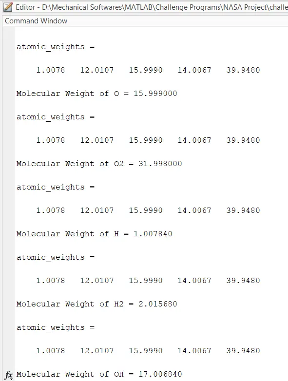
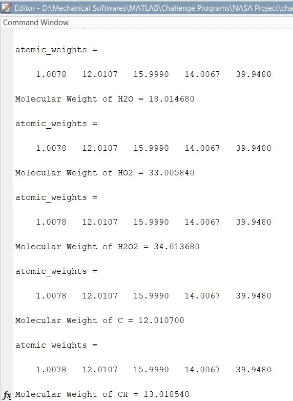
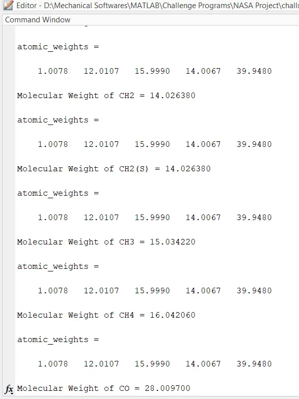
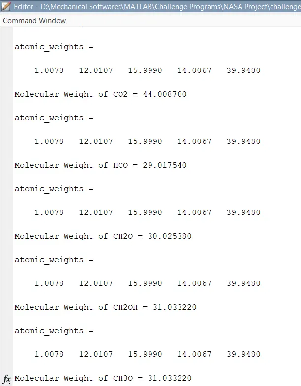
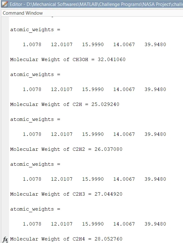
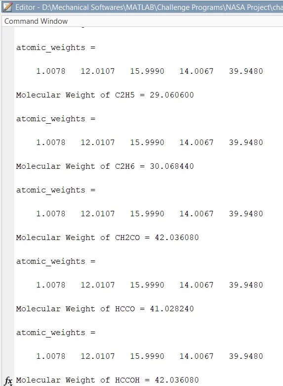
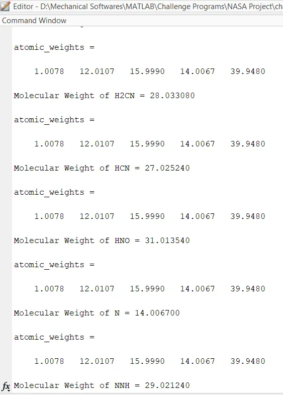
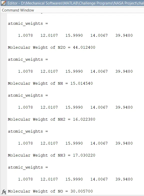
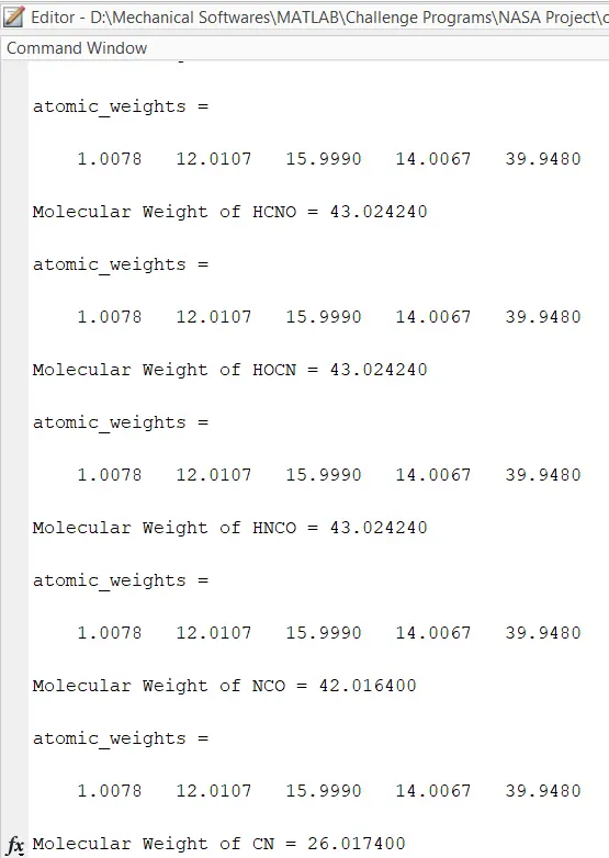
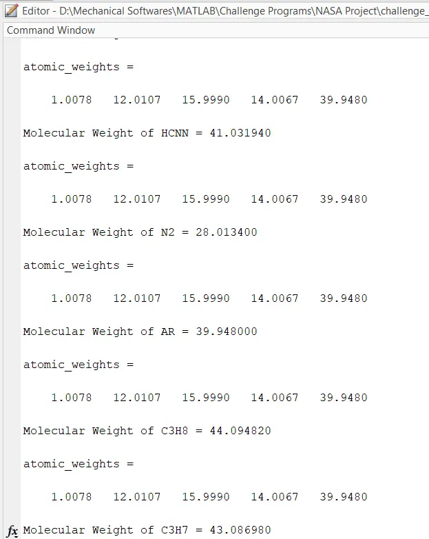
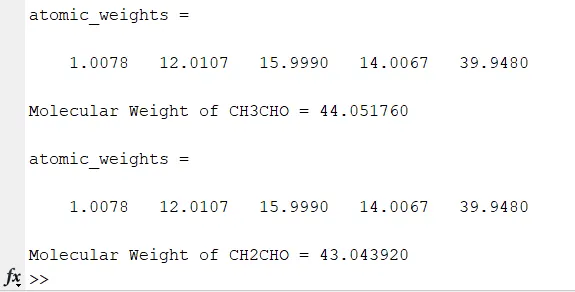
Calculate the molecular weight of each species and display it in the command window.
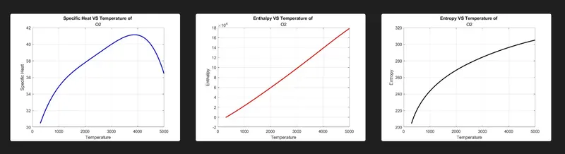
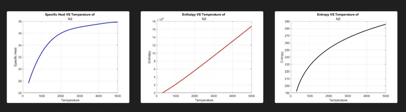
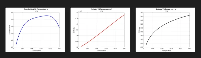
Plot the Cp, Enthalpy, and Entropy for the local temperature range (low temperature: high temperature) specific for each species.
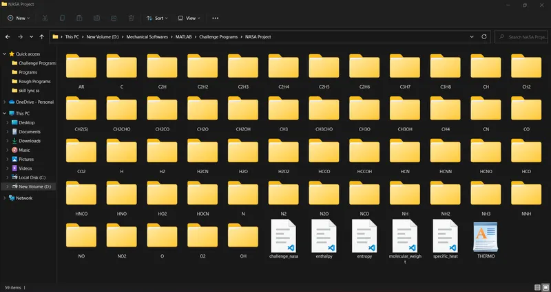
Save the plots as images with appropriate names and dump them in separate folders for each species with a suitable name. All these should be generated automatically.

THEORY:

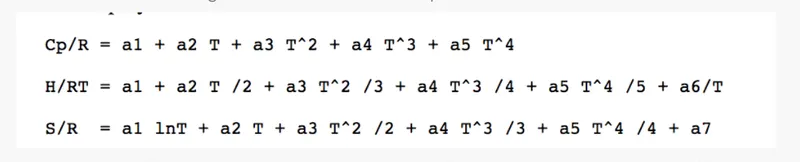
The formula of Specific Heat, Enthalpy, Entropy is bellowed:

Specific Heat: the quantity of heat required to raise the temperature of one gram of a substance by one Celsius degree. The units of specific heat are usually calories or joules per gram per Celsius degree. For example, the specific heat of water is 1 calorie (or 4.186 joules) per gram per Celsius degree. It is denoted as Cp.
Enthalpy: The sum of the internal energy and the product of the pressure and volume of a thermodynamic system. Enthalpy is an energy-like property or state function. It has the dimensions of energy (and is thus measured in units of joules or ergs), and its value is determined entirely by the temperature, pressure, and composition of the system and not by its history. In symbols, the enthalpy, H, equals the sum of the internal energy, E, and the product of the pressure, P, and volume, V, of the system: H = E + PV. According to the law of energy conservation, the change in internal energy is equal to the heat transferred to, less the work done by, the system. If the only work done is a change of volume at constant pressure, the enthalpy change is exactly equal to the heat transferred to the system. When energy needs to be added to a material to change its phase from a liquid to a gas, that amount of energy is called the enthalpy (or latent heat) of vaporization and is expressed in units of joules per mole. It is denoted as H.
Entropy: a thermodynamic quantity representing the unavailability of a system's thermal energy for conversion into mechanical work, often interpreted as the degree of disorder or randomness in the system. The second law of thermodynamics says that entropy always increases with time. It is denoted as S.
In the above three equations, where a1, a2, a3, a4, a5, a6, and a7 are the numerical coefficients supplied in NASA thermodynamic files. The first 7 numbers starting on the second line of each species entry (five of the second line and the first two of the third line) are the seven coefficients (a1 through a7, respectively) for the high-temperature range (above 1000 K, the upper boundary is specified on the first line of the species entry). The remaining seven numbers are the coefficients (bl through b7, respectively) for the low-temperature range (below 1000 K, the lower boundary is specified on the first line of the species entry).
Parsing: in computer languages refers to the syntactic analysis of the input code into its components parts in order to facilitate the writing of compilers and interpreters. It can be used to describe split or separation. Parsing a file means reading in a data stream of some sort and building an in-memory model of the semantic content of that data. This aims at facilitating performing some kind of transformation on the data.

PROCEDURE:

Function Code for Specific Heat (cp):

function [cp] = specific_heat(a1,a2,a3,a4,a5,a8,a9,a10,a11,a12,tmid,T,R)

% Finding Specific Heat with Low Temperature Variables
if T<=tmid
    cp = (a8+(a9*T)+(a10*T.^2)+(a11*T.^3)+(a12*T.^4))*R;
else
    cp = (a1+(a2*T)+(a3*T.^2)+(a4*T.^3)+(a5*T.^4))*R; 
end

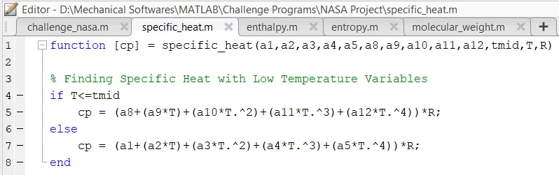
Line 1 - Writing the function command for cp.
Line 4 to 8 - Introducing if and else command to the conditional statement to pass the right coefficients to find Specific heat and ending the function with an end command.

Function Code for Enthalpy (H):

function [H] = enthalpy(a1,a2,a3,a4,a5,a6,a8,a9,a10,a11,a12,a13,tmid,R,T)

% Finding Specific Heat with Low Temperature Variables
if T<=tmid
    H = (a8+(a9*T/2)+(a10*(T.^2)/3)+(a11*(T.^3)/4)+(a12*(T.^4)/5)+(a13./T))*R.*T;
else
    H = (a1+(a2*T/2)+(a3*(T.^2)/3)+(a4*(T.^3)/4)+(a5*(T.^4)/5)+(a6./T))*R.*T;
end

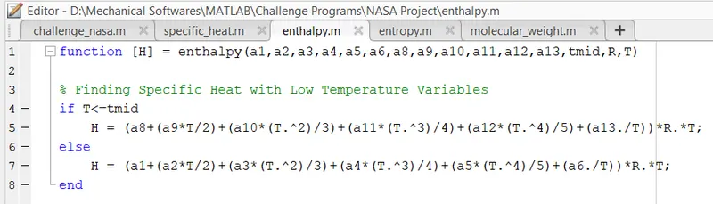
Line 1 - Writing the function command for H.
Line 4 to 8 - Introducing if and else command to the conditional statement to pass the right coefficients to find Enthalpy and ending the function with an end command.

Function Code for Entropy (S):

function [S] = entropy(a1,a2,a3,a4,a5,a7,a8,a9,a10,a11,a12,a14,tmid,T,R)

% Finding Specific Heat with Low Temperature Variables
if T<=tmid
    S = ((a8*log(T))+(a9*T)+(a10*(T.^2)/2)+(a11*(T.^3)/3)+(a12*(T.^4)/4)+a14)*R;
else
    S = ((a1*log(T))+(a2*T)+(a3*(T.^2)/2)+(a4*(T.^3)/3)+(a5*(T.^4)/4)+a7)*R;
end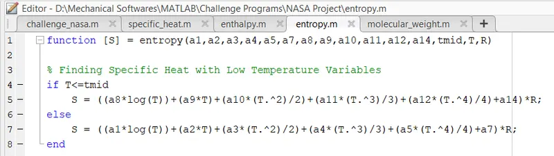

Line 1 - Writing the function command for S.
Line 4 to 8 - Introducing if and else command to the conditional statement to pass the right coefficients to find Entropy and ending the function with an end command.

Main Code to Parse the NASA thermodynamic data file and make plots:

% File Prasing - NASA Thermodynamic Data
clear all
close all
clc

% Opening The Thermodynamic data file
f1 = fopen('THERMO.dat','r');

% Skipping the First Line
fgetl(f1);

% For the Global Temperatures
temps = fgetl(f1);
temps = str2num(temps);

global_low_temp = temps(1);
global_mid_temp = temps(2);
global_high_temp = temps(3);

% For creating an array for these temperatures
T = linspace(global_low_temp,global_high_temp,500);

% The Universal Gas Constant
R = 8.314;

% Skipping next 3 Lines because the line starts with '!' and it can be ignored
for i = 1:3
    fgetl(f1)
end

% Lets Start the Sorting of the values
for i = 1:53
    
    % Creating an array for species
    tline = fgetl(f1);
    A = strsplit(tline,' ');
    
    % Let the species be 
    species = A{1};
    
    % Local Temperatures
    tlow = str2num(A{end-3});
    thigh = str2num(A{end-2});
    tmid = str2num(A{end-1});
    
    % Fining the Coefficients
    % Line 1
    tline1 = fgetl(f1);
    pos1 = findstr(tline1,'E');
    
    % For the Higher Coefficients
    a1 = str2num(tline1(1:pos1(1)+3));
    a2 = str2num(tline1(pos1(1)+4:pos1(2)+3));
    a3 = str2num(tline1(pos1(2)+4:pos1(3)+3));
    a4 = str2num(tline1(pos1(3)+4:pos1(4)+3));
    a5 = str2num(tline1(pos1(4)+4:pos1(5)+3));
    
    % Line 2
    tline2 = fgetl(f1);
    pos2 = findstr(tline2,'E');
    a6 = str2num(tline2(1:pos2(1)+3));
    a7 = str2num(tline2(pos2(1)+4:pos2(2)+3));
    
    % For the Lower Coefficents
    a8 = str2num(tline2(pos2(2)+4:pos2(3)+3));
    a9 = str2num(tline2(pos2(3)+4:pos2(4)+3));
    a10 = str2num(tline2(pos2(4)+4:pos2(5)+3));
    
    % Line 3
    tline3 = fgetl(f1);
    pos3 = findstr(tline3,'E');
    a11 = str2num(tline3(1:pos3(1)+3));
    a12 = str2num(tline3(pos3(1)+4:pos3(2)+3));
    a13 = str2num(tline3(pos3(2)+4:pos3(3)+3));
    a14 = str2num(tline3(pos3(3)+4:pos3(4)+3));
    
    % For the Calculation of Specific Heat
    cp = specific_heat(a1,a2,a3,a4,a5,a8,a9,a10,a11,a12,tmid,T,R);
    
    % For the Calculation of Enthalpy
    H = enthalpy(a1,a2,a3,a4,a5,a6,a8,a9,a10,a11,a12,a13,tmid,R,T);
    
    % For the Calcualtion of Entropy
    S = entropy(a1,a2,a3,a4,a5,a7,a8,a9,a10,a11,a12,a14,tmid,T,R);
    
    % Chaning the Directory
    cd('D:Mechanical SoftwaresMATLABChallenge ProgramsNASA Project')
    
    % Creating Newfolder for Species
    mkdir(species)
    
    % Changing Directory 
    cd(species)
    
    % Plotting
    
    figure(1)
    plot(T,cp,'linewidth',2,'color','b')
    xlabel('Temperature')
    ylabel('Specific Heat')
    title('Specific Heat VS Temperature of ',sprintf('%s',species))
    grid on
    saveas(figure(1),'cp vs T.jpg')
    
    figure(2)
    plot(T,H,'linewidth',2,'color','r')
    xlabel('Temperature')
    ylabel('Enthalpy')
    title('Enthalpy VS Temperature of ',sprintf('%s',species))
    grid on
    saveas(figure(2),'H vs T.jpg')
    
    figure(3)
    plot(T,S,'linewidth',2,'color','k')
    xlabel('Temperature')
    ylabel('Entropy')
    title('Entropy VS Temperature of ',sprintf('%s',species))
    grid on
    saveas(figure(3),'S vs T.jpg')
    
    % Coming back to the Program Directory
    cd('D:Mechanical SoftwaresMATLABChallenge ProgramsNASA Project')
    
    % Calculating Molecular Weight of Species
    M = molecular_weight(species);
    
end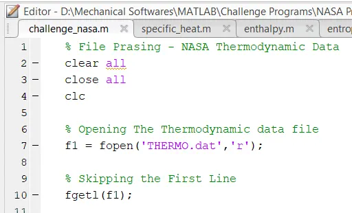

clear all - To clear all variables from the current workspace
close all - close all figures whose handles are visible.
clc - clears all the text from the Command Window.
fopen - It opens the file, filename, for binary read access, and returns an integer file identifier equal to or greater than 3.
fgetl - fgetl returns an output that displays in one line.
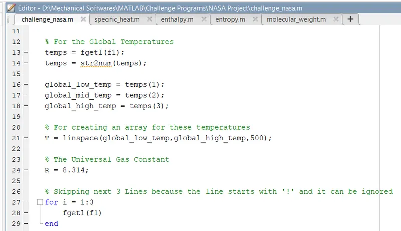
Line 14 to 19 - Read and store the global temperature values into separate variables.
str2num - converts a character into an array or string scalar to a numeric matrix.
Line 21 - Creating an array for Temperature.
linspace - The linspace function generates linearly spaced vectors.
Line 24 - Writing Universal Gas Constant value R.
Line 28 to 30 - Skipping the next 3 lines using fgetl command.
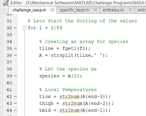
Line 35 to 39 - Creating a variable for storing species names.
strsplit - It is used to split a string. We should enter the string ID and delimiter.
{A1} - It is used for indexing in cell arrays. After string splitting A becomes a cell array.
Line 42 to 44 - Defining local temperatures.
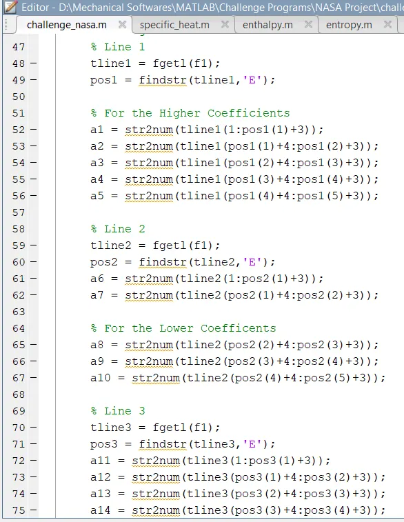
Line 48 to 75 - Extracting and stores coefficients from the dat file.
findstr - It is used to find a particular string in a collection of strings. We should define the string array and letter that need to be found inside that function. The command gives the position of the letters in the string.
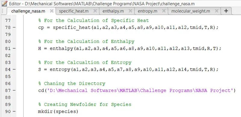
Line 78 - Calling specific_heat function for storing the values of specific heats of species into cp.
Line 81 - Calling enthalpy function for storing the values of enthalpies of species into H.
Line 84 - Calling entropy function for storing the values of entropies of species into S.
cd - To change directory.
mkdir - It is used to create a new folder. The name of the folder should be mentioned inside the brackets.
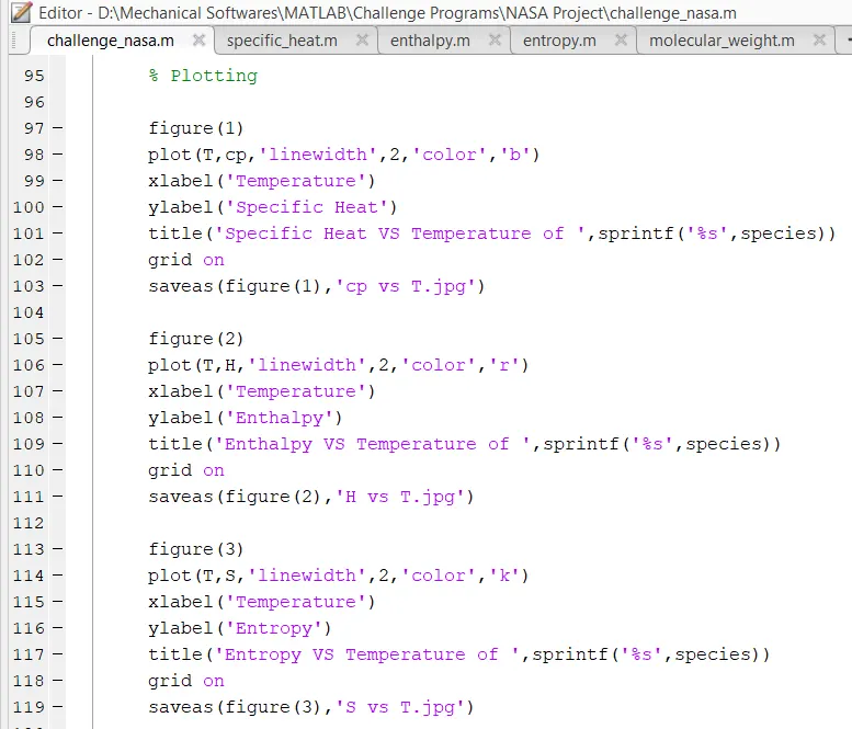
Line 97 to 116 - Plotting graphs of cp vs T, H vs T, and S vs T.
figure - To create 3 different figures of plots.
plot - The plot function in Matlab is used to create a graphical representation of some data.
linewidth - To give width to the Graphical representing line.
color - To give the required color to the Graphical representing a line.
xlabel- To label x-axis.
ylabel- To label the y-axis.
title - To add a title to a plot.
saveas - saveas(fig, filename) saves the figure specified by fig to file filename.
Line 122 - Calling the cd command to change the Program Directory.
Line 125 - Calling molecular_weight function for storing the values of molecular weights into M.

Function Code for Molecular weight of species:

function [W] = molecular_weight(species)

atomic_names = ['H', 'C', 'O', 'N', 'Ar'];
atomic_weights = [1.00784, 12.0107, 15.999, 14.0067, 39.948]
W=0;

for i=1:length(species)
    for j=1:length(atomic_names)
        if species(i)==atomic_names(j)
            W=W+atomic_weights(j);
            position = j;
        end
    end
    n=str2num(species(i));
    if n>=1
        W=W+atomic_weights(position)*(n-1);
    end
end
fprintf('Molecular Weight of %s = %f',species,W)
disp(' ')
end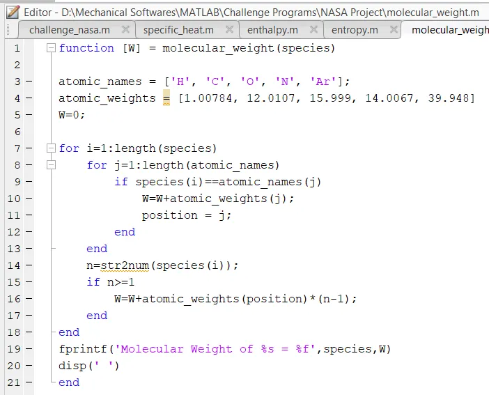

Line 3 - Since all the 53 species are made of H, C, ON, Ar only, we are creating a string array for these.
Line 4 - Creating an array for the atomic weights of these five atoms.
Line 7 to 18 - Introducing loops and conditional statements to calculate the molecular weight of species.
fprintf - The fprintf command displays formatted text centered on the icon and can display format specifier along with the contents of variables.
disp - disp(X) displays the value of variable X without printing the variable name.

Errors faced while Programming:

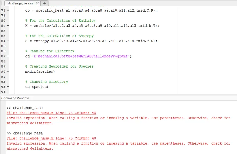
There were many errors like this these errors typos made by me in the function files and the main program files, the errors were removed by making the required changes in the code.
The other major error I faced was with the opening file directory, making a new folder, and everything, it took me a while to figure things out, I researched and learned the proper way to do it.

RESULTS:

Plots of O2:

Plots of N2:

Plots of Co2:

Command Window Results of Molecular Weight:

Screenshot of the Folder Created automatically:

Drive link of the Entire Folder: https://drive.google.com/drive/folders/1obfvbHl457fky4whrDro8E5S7JWCWte4?usp=sharing

CONCLUSION:

Hence, we conclude that using the above MATLAB COde. The required data was extracted from the NASA thermodynamics data file. Used this data for the calculation of specific heat, enthalpy, and entropy. Also, plot the graph for the above properties vs local temperature. The Molecular weight was also calculated. A new folder was created to save all data.

REFERENCES:

Parsing NASA Thermodynamic Data using MATLAB

Ship work like this
in your own course.

Talk to a career counsellor

Ship work like thisin your own course.

Talk to a career counsellor

Ship work like this
in your own course.