Creating an Otto Cycle P-V Diagram and Calculating its Efficiency using MATLAB.
Aim: TO visualize the P-V Diagram of Otto Cycle and to calculate thermal efficiency using Matlab.
Equation required For solving the problem:
Here this equation is used to show the relationship between crank angle and volume inside crank angle and volume inside the crank chamber

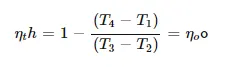
And another governing equation is this, the formula for thermal efficiency,
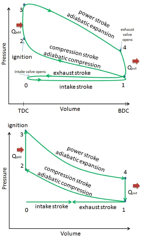
Objective: To calculate the Thermal Efficiency and plot the P-V diagram of the Otto cycle.
Theory:
- Process 1-2 mass of air is drawn into the cylinder.
- Process 2-3 is an isentropic compression, as the piston moves from BDC (bottom dead center) to TDC (top dead center).
- Process 3-4 is a constant volume heat addition in this the air-fuel mixture inside the cylinder pushes the piston from TDC to BDC.
- Process 4-5 is an isentropic expansion (Power stroke). That is, the air-fuel mixture gets ignited by the spark plug.
- Process 5-6 is constant volume heat rejection; in this process the cycle is complete and it's the blowdown.
- Process 6-1 the mass of air is released into the atmosphere in a constant pressure process.
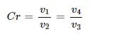
Compression Ratio: Compression ratio (cr) is the ratio of total cylinder volume to the clearance volume
Now that we know the basic term, let us derive the expression for and. These expressions will be useful for us to derive the expression for air standard efficiency of the Otto cycle. For finding, we take process 1-3 and for finding, we take process 3-4.
Process 1-2: This process is an isentropic (reversible adiabatic) process. For this process, the relation between T and V is:
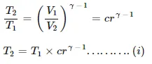
Process 3-4: This is also an isentropic process. The relation between T and V in the process is similar to the relation between T and V in process 1-2.
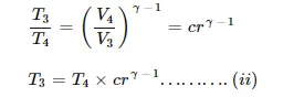
Air-standard Efficiency (thermal efficiency) of Otto cycle,
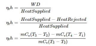
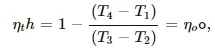
Thermal Efficiency can be calculated by using different values of temperature. Thermal efficiency can also be calculated by using the relation:
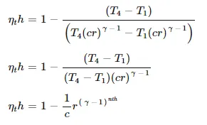
Writing down the required Function Code:
function [V] = challenge_engine_kinematics(bore, stroke, con_rod, cr, start_crank, end_crank)

% Crank Pin Radius
a = stroke/2;
% Ratio of Connecting Rod and Crank Pin Radius.
R = con_rod/a;
% Swept Volume Calculation
v_s = (pi/4)*bore^2*stroke;
% Clearance Volume Calculation
v_c = v_s/(cr-1);
% Creating an array for diffrent theta values
theta = linspace(start_crank,end_crank,100)
% Combustion Volume Formula Calculation
term1 = 0.5*(cr-1);
term2 = R +1 - cosd(theta);
term3 = (R^2 - sind(theta).^2).^0.5;

V = (1 + term1*(term2 - term3)).*v_c;

end
Code Explanation:
- So in the above code, I have created a function named "challenge_engine_kinematics" which has the ability to take input values and assign value to the output array.
- Then in inputs, I wrote down the formula for Crankpin radius and Ratio of Connecting Rod and Crankpin Radius.
- Then in the next steps, I wrote the formula for the calculation of the Swept Volume and Clearance Volume.
- For the different values of theta, I created an array using linspace command.
- In the final step, I wrote down the formula for the calculation of the combustion volume, while writing this down I split the main formula into 3 small parts and named each part as term1, term2, term3 and finally combined all the terms into a single main formula.
Writing down the required code for PV Diagram and Thermal Efficiency:
clear all
close all
clc

% Inputs
gama = 1.4;
t3 = 2300;

% State Variable values for Stage 1
p1 = 101325;
t1 = 500;

% Engine Geometric Parameters
bore = 0.1;
stroke = 0.1;
con_rod = 0.15;
cr = 12;

% Formula for calculation of Swept Volume and Clearnace Volume
v_swept = (pi/4)*bore^2*stroke;
v_clearance = v_swept/(cr-1);

% Volume at satge 1 and 2
v1 = v_swept + v_clearance;
v2 = v_clearance;

% State Variable values for Stage 2
% p2v2^gama = p1v1^gama | p2 = p1(v1/v2)^gama = p1*cr^gama
p2 = p1*cr^gama;

% Temperature at point 2
% p1v1/t1 = p2v2/t2 | t2 = p2*v2*t1(p1*v1)

t2 = p2*v2*t1/(p1*v1);

% For Constant C
constant_c = p1*v1^gama;

% For compresion Stroke Volume and Pressure Calculation
V_compression = challenge_engine_kinematics(bore, stroke, con_rod, cr,180,0);
P_compression = constant_c./V_compression.^gama;

% State Variable values for Stage 3
v3 = v2;

% Pressure at point 3
% p3v3/t3 = p2v2/t2 | p3 = p2*t3/t2
p3 = p2*t3/t2;

% For Constant C
constant_c = p3*v3^gama;

% For compresion Stroke Volume and Pressure Calculation
V_expansion = challenge_engine_kinematics(bore, stroke, con_rod, cr,0,180);
P_expansion = constant_c./V_expansion.^gama;

% State Variable values for Stage 4
v4 = v1;

% p3v3^gama = p4v4^gama | p4 = p3(v3/v4)^gama
p4 = p3*(v3/v4)^gama;

% Formula for Thermal Efficiency
thermal_efficiency = (1-(1/cr^(gama - 1)))*100;

% Plotting of P-V Diagram
hold on
plot(V_compression, P_compression)
plot([v2,v3],[p2,p3])
plot(V_expansion, P_expansion)
plot([v4,v1],[p4,p1])
title ('Otto Cycle P-V Diagram')
xlabel('Volume')
ylabel('Pressue')
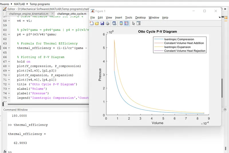
legend('Isentropic Compression','Constant Volume Heat Addition','Isentropic Expansion','Constant Volume Heat Rejection')
Code Explanation:
- Started the code with clear all, close all, and clc.
- Then I wrote the input values of "gama" and "t3".
- Now I wrote down values for State Variables at Stage 1 "p1" and "t1".
- After this, I included the Engine Geometric Parameters, which included the values of the "bore", "stroke", "connecting rod" and "compression ratio".
- After this, I wrote the formula for the calculation of the "Swept Volume" and "Clearance Volume".
- Then I wrote down the formula for volume at stages 1 and 2; "v1" and "v2".
- Now again values for State Variables but at Stage 2 wrote the formula for "p2".
- Then the formula for the temperature at stage 2 "t2".
- Now formula for the "constant_c", now as we got the formula for the "constant_c" we can now easily calculate the "Compression Stroke Volume" and "Compression Stroke Pressure" so wrote down those formulas also.
- Now again values for State Variables but at Stage 3 now "v3".
- The formula for "Pressure" at point 3 and "Constant_c". As we got the "Constant_C" we can now easily calculate the "Expansion Stroke Volume" and "Expansion Stroke Pressure" so wrote down those formulas also.
- For the final State Variable stage, 4 wrote formulas of "v4" and "p4".
- Now for the "Calculation of the Thermal Efficiency" wrote the formula for the same.
- Towards the final part i.e. the plotting of the P-V Diagram started with the "hold on" command followed by the plotting of the points (V_compression, V_expansion,v1,v2,v3,v4 and P_compression, P_expansion,p1,p2,p3,p4) also give the title and x-axis and y-axis names. I even included the legend command for a little more detail adding purpose.
Results of the Code:
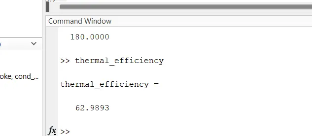
Output for Thermal Efficiency of Engine:
The plot of the P-V Diagram:
The Errors I faced while Programming:
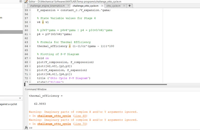

I faced the above two errors actually, it was a small typo on my function file "challenge_engine_kinematics" I made a typo in writing the formula for Ratio of Connecting Rod and Crank Pin Radius the formula I wrote was "R = con_rod/2;" which was wrong as the correct formula was "R = con_rod/a;"