Solving second order ODEs using MATLAB to simulate motion of simple pendulum.

Aim:- To write a matlab program to simulate motion of simple pendulum

Engineering Data :-

The given 2nd order differential equation is the governing equation for simple pendulum having damping also.

All the units are in SI. Given inputs are

Length of pendulum rod = 1 m

Acceleration due ro gravity (g) = 9.8 m/s^2

Mass of the pendulum (m) = 1 kg

Damping Coefficient = 0.05

Initial Conditions are

Displacement = 0, Velocity = 3 rad/sec, Time interval is from 0 to 20 sec.

Code:-

clear all
close all
clc
%input parameters 
g= 9.81;
b= 0.05;
l = 1;
m=1;

%initial conditions
theta_0 = [0;3];

% Time limits for intergration 
time_span = linspace(0,20,200);

%Created a ODE function and calling it down for the results
[t, values] = ode45(@(t, theta) odefunction(t, theta, g, b, m, l), time_span, theta_0); 

%Plotting the graph which shows the displacement and velocity of the
%pendulum with respect to time for given initial conditions and damping
%coefficient
figure(1)
plot(t,values(:,1)) 
hold on
 plot(t, values(:,2))
 xlabel('time')
 legend('Displacement', 'velocity')
 
 %For creating animations loop is created
ct=1 ;
 for i= 1:length(time_span)
     %To create the distance covered by end of pendulum in both x-axis and
     %y-axis
     X1 = l* sin(values(i,1));
     Y1= -l* cos(values(i,1));
     %To create pendulum starting point
      X0=0;
      Y0=0;
    %To create another figure for the pendulum animation
     figure(2)
     plot([-1,1], [0,0], 'linewidth',4,'color','r') 
     hold on
     axis([-2 2 -2 2])
     
     %To create fixed support for pendulum
     line([X0 X1], [Y0 Y1],'linewidth',3,'color','y')   
     
     %To create the pendulum bob using O as marker with larger size
     plot(X1,Y1, 'o', 'markersize',10,'markerfacecolor','b')  
     legend ('Fixed Support', 'pendulum rod', 'pendulum bob')
     pause(0.01)
     hold off 
     M(ct)=getframe(gcf);
 ct=ct+1;
 end
 %To save the previously captured frames as a single video file
 movie(M);
 videofile= VideoWriter('pendulum', 'Uncompressed AVI');
 open(videofile)
 writeVideo(videofile,  M)
 close(videofile)

Function code :-

function [dtheta_dt] = odefunction(t, theta, g, b, m, l)


%To assign initial conditions in the form of matrix from main code
theta1 = theta(1); 
theta2 = theta(2);

dtheta1_dt = theta2;
dtheta2_dt = (-b/m)*theta2 -(g/l)*sin(theta1);
dtheta_dt = [ dtheta1_dt; dtheta2_dt];
end

Ode45:-

Ode45 is a inbuilt matlab command used to solve first order diferential equations. If the given equation has order more than 1, lets say 'n' it must be simplified into n number of first order differential equations and after that used in matlab for calculations.

The syntax of ode45 is shown below :-

[t,y] = ode45(@(t,y) 2*t, tspan, y0) and the syntax used in our code is

[t, values] = ode45(@(t, theta) odefunction(t, theta, g, b, m, l), time_span, theta_0);

The syntax is divided into mainly 4 elements. At first we have to adress the dependent and independent variable, in the above syntax it is theta and time so it is @(t, theta). In the second part we have to call the function for calculation if required by the complexity of the problem. After that in 3rd and 4th part we have to mention the initial conditions for dependent and independent variables. In the given problem 'time' is independent and 'theta' is dependent variable.

Steps to create Animation:-

The steps followed in the above code are

1. To count the frames above and below the for loop by using ct.

2. The counted frames are to be captured by the following command M(ct)=getframe(gcf);

3. Then assign the counted frames to a variable, Create an empty video file and dump the captured frames to the empty video by following the steps down below

Results and Observations :-

By compiling the above code we get the following graph and animation. Animation is shared by google drive. (Due to size of the video, the animation is made faster)

Link to Animation :- usp=sharinghttps://drive.google.com/file/d/14OZ71aAWAGpL9Hj_ei1rCG8ioi4DmqWV/view? usp=sharing

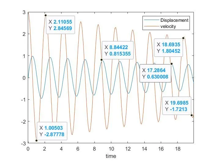
Hence from the above graph it is observed that the motion of pendulum is Simple Harmonic, the velocity and displacement of the pendulum is decreasing with respect to time because of the damping provided. The more the damping the faster the pendulum comes to rest.