Simulation of Rankine Cycle using MATLAB

Aim :- To create rankine cycle simulator in MATLAB and calculate the following

1. Net Work Output

2. Back Work Ratio

Rankine Cycle :-

All units are in SI.

The processes involved are:

1-2 : Constant Pressure Heat Addition in Boiler
2-3 : Isentropic Expansion in Turbine
3-4 : Constant Presuure Heat Rejection by Condenser
4-1 : Pump work for transfer of Condensed Water to Boiler

Net Work Output = Turbine Work - Pump Work

Back work Ratio = Negative work in cycle/ Positive work in cycle

Code :-

clear all
close all 
clc 

%All units for the problem are in SI. 
%For printing of processes in Rankine Cycle 
fprintf('RANKINE CYCLE SIMULATOR  n')
fprintf(' 1-2 : Constant Pressure Heat Addition in Boiler n')
fprintf(' 2-3 : Isentropic Expansion in Turbine n')
fprintf(' 3-4 : Constant Presuure Heat Rejection by Condenser n')
fprintf(' 4-1 : Pump work for transfer of Condensed Water to Boiler n')

%Input Conditions for the Rankine Cycle 
P2 = input('Pressure at the inlet of turbine (P2) (in bar): ');
P3 = input('Pressure at the outlet of turbine(P3) (in bar): ');
T2 = input('Temperature at inlet of turbine(T2) (in Celcius): ');

%Conditions at the inlet of the turbine which are outlet of Boiler
%Hf refers to Enthalpy at saturated liquid and Hg refers to enthalpy at
%saturated vapour followed by state point.  Same notations apply for entropy also. 
H2= XSteam('h_pt', P2,T2);
S2 = XSteam('s_pt', P2, T2);
Hf2 = XSteam('hL_p', P2);
Hg2 = XSteam('hV_p', P2);
Sf2 = XSteam('sL_p', P2);
Sg2 = XSteam('sV_p', P2);
Ts2 = XSteam('Tsat_p',P2); 

%Conditions at the outlet of turbine which are inlet to condenser 

Sf3 = XSteam('sL_p', P3);
Sg3 = XSteam('sV_p', P3);
S3 = S2; 
x = (S3 - Sf3)/(Sg3-Sf3);  %x denotes Dryness fraction x = mass of vapour/ (mass of vapour+mass of liquid)
Hf3 = XSteam('hL_p', P3);
Hg3 = XSteam('hV_p', P3);
H3 = Hf3 + x*(Hg3-Hf3);
T3 = XSteam('T_ph', P3, H3);
Ts3 = XSteam('Tsat_p',P3);

%Conditions at the exit of Condenser which are inlet to pump 
 T4 = T3;
 P4 = P3;
 H4 = Hf3;
 S4 = Sf3;
 
 %Conditions at exit of pump which are  inlet to Boiler 
 
 P1 = P4;
 S1 = S4;
 H1 = XSteam('h_ps', P1, S1);
 T1 = XSteam('T_ps', P1, S1);

 %Calculating Turbine Work output 
 Turbine_Work = H2-H3;
 
 %Calculating Pump Work, x.vg4 is too small, so we can ignore it from
 %Engineering point of view 
  vf4 = XSteam('vL_p', P4);
 Pump_Work = vf4*(P2-P3)*10^2;
 
 %Calculating the required Parameters given in Problem 
 Net_Work_Output = Turbine_Work - Pump_Work;   
 
 %Back work Ratio = -ve work in cycle/ +ve work in cycle 
 Back_Work_Ratio = Pump_Work / Turbine_Work;
 
 %For printing of Parameters at each state. 
fprintf('n FINAL RESULTS n')
fprintf( '   At state point 1 : n')
fprintf(' Pressure in Bar           =   %.3fn', P1)
fprintf(' Temperature in C       =   %.3fn',T1)
fprintf( ' Enthalpy in KJ/kg      =   %.3f n', H1)
fprintf( ' Entropy in KJ/kg-K   =   %.3fn', S1)

fprintf( '  n At state point 2 : n')
fprintf(' Pressure in Bar           =   %.3fn', P2)
fprintf(' Temperature in C       =   %.3fn',T2)
fprintf( ' Enthalpy in KJ/kg      =   %.3f n', H2)
fprintf( ' Entropy in KJ/kg-K   =   %.3fn', S2)

fprintf( '  n At state point 3 : n')
fprintf(' Pressure in Bar           =   %.3fn', P3)
fprintf(' Temperature in C       =   %.3fn',T3)
fprintf( ' Enthalpy in KJ/kg      =   %.3f n', H3)
fprintf( ' Entropy in KJ/kg-K   =   %.3fn', S3)

fprintf( ' n  At state point 4 : n')
fprintf(' Pressure in Bar           =   %.3fn', P4)
fprintf(' Temperature in C       =   %.3fn',T4)
fprintf( ' Enthalpy in KJ/kg      =   %.3f n', H4)
fprintf( ' Entropy in KJ/kg-K   =   %.3fn', S4)

%Printing of Required answers asked in Question 
fprintf(' n Net Work Output in KJ/kg = %.3fn', Net_Work_Output)
fprintf(' Back Work Ratio = %.7fn', Back_Work_Ratio)

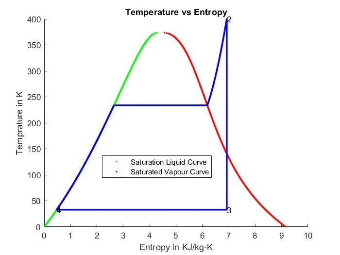
%Plotting of Temperature - Enthalpy Diagram
%For creating graph, by using linspace command we created temperature
%iterations
Temperature = linspace(0,400,500); 
figure(1)
hold on
%Using for loop command for plotting saturation curve by taking data from
%XSteam library 
for i = 1 : length(Temperature)
 plot(XSteam('sL_T',Temperature(i)),Temperature(i),'.','color','g')
 plot(XSteam('sV_T',Temperature(i)),Temperature(i),'.','color','r')
end
%Plotting the state parameters 
plot([S2 S3],[T2 T3],'linewidth',2,'color','b')
if x>1
 T4 = Ts3;
plot([S3 Sg3 S4 S1],[T3 Ts3 T4 T1],'linewidth',2,'color','b')
 T3 = Ts3;
else
 plot([S3 S4 S1],[T3 T4 T1],'linewidth',2,'color','b')
end
l = linspace(T2,T3,1000);
for i = 1 : length(l)
 plot(XSteam('s_pT',P2,l(i)),l(i),'.','color','b')
end
plot([Sf2 Sg2],[Ts2 Ts2],'linewidth',2,'color','b')
xlabel('Entropy in KJ/kg-K')
ylabel('Temprature in K')
title('Temperature vs Entropy')
legend('Saturation Liquid Curve', 'Saturated Vapour Curve')
%Marking state points on Graph
text(S1, T1, '1')
text(S2, T2,'2')
text(S3, T3, '3')
text(S4, T4, '4')

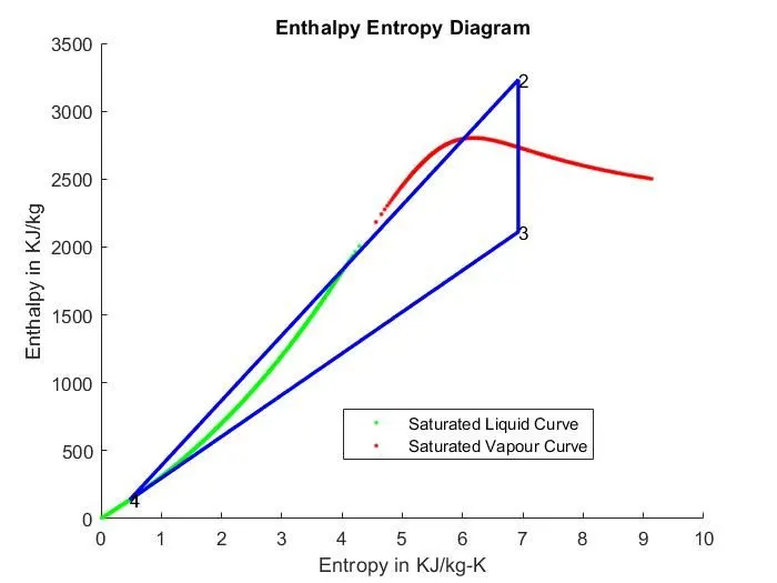
%Plotting of Enthalpy - Entropy Diagram 
figure(2) 
hold on 
%Using for loop command for plotting saturation curve by taking data from
%XSteam library 
for i = 1 : length(Temperature)
 plot(XSteam('sL_T',Temperature(i)),XSteam('hL_T',Temperature(i)),'.','color','g')
 plot(XSteam('sV_T',Temperature(i)),XSteam('hV_T',Temperature(i)),'.','color','r')
end

plot([S1 S2 S3 S4 S1],[H1 H2 H3 H4 H1],'linewidth',2,'color','b')
xlabel('Entropy in KJ/kg-K')
ylabel('Enthalpy in KJ/kg')
title('Enthalpy Entropy Diagram')
legend('Saturated Liquid Curve', 'Saturated Vapour Curve')

%Marking State points on curve 
text(S1, H1, '1')
text(S2, H2,'2')
text(S3, H3, '3')
text(S4, H4, '4')

Code explanation and logic:-

1. Provided XSteam library must be in same folder where matlab is working on.

2. By using XSteam('hV_p', P1) etc, like commands are used to extract state points and saturation curves. For the exact commands which are required open XSteam.m file in matlab. It shows how to use commands.

3. By applying basic engineering calculations for rankine cycle, the parameters like Enthalpy, Entropy and temperature is evaluated for each state points. Formulas and steps for doing it are mentioned in the above code with comments.

4. Graphs are plotted by using the above procedure.

5. By using input commands, this code can work for different intital pressure and temperature conditions where water is the working medium in the cycle.

Results and Observations :-

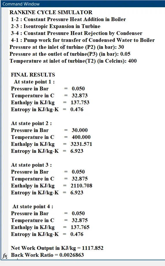
Hence Rankine Cycle is simulated and found the properties at each state point as shown below.

Also found the Net Work Output and Back WorK Ratio.

References :-

http://matlab.cheme.cmu.edu/2011/10/31/matlab-meets-the-steam-tables/

Engineering Thermodyamics by P.K. Nag.