Week 3 - Solving second order ODEs

AIM :

To find the second order Ordinary Differential Equation using MATLAB.

THEORY :

An ordinary differential equation (also abbreviated as ODE), in Mathematics, is an equation which consists of one or more functions of one independent variable along with their derivatives. A differential equation is an equation that contains a function with one or more derivatives. But in the case ODE, the word ordinary is used for derivative of the functions for the single independent variable.

In Engineering, ODE is used to describe the transient behavior of a system. A simple example is a pendulum

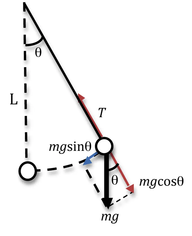
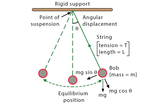
A simple pendulum can be described as a device where its point mass is attached to a light inextensible string and suspended from a fixed support. The vertical line passing through the fixed support is the mean position of a simple pendulum. The vertical distance between the point of suspension and the centre of mass of the suspended body (when it is in mean position) is called the length of the simple pendulum denoted by L. This form of the pendulum is based on the resonant system having a single resonant frequency.

GOVERNING EQUATIONS :

`(d^2theta)/dt^2 + b/m * (d theta)/dt + g/L * sin theta = 0` ---------------(1)

Where ,

`theta` is the angle made by the movable link with the vertical axis.

L is the length of the movable rod.

m is the mass of bob,

b is the damping coefficient of the system.

To solve this ODE in MATLAB Program, we need to reduce the order of equation to a lower order, say (`theta = theta_1`).

which implies,

`(d(theta))/dt = (d(theta_1))/dt = theta_2` --------------(2)

Therefore,

`(d^2(theta))/dt^2 = (d^2(theta_1))/dt^2 = (d theta_2)/dt` ---------------------------(3)

By putting the values (2) and (3) in (1), we get,

`(d^2theta_1)/dt + b/m* (d(theta_1))/dt + g/L* sin theta_1 = 0`

`implies (d(theta_2))/dt + b/m*(theta_2) + g/L * sin theta_1 = 0`

`implies (d(theta_2))/dt = - b/m*(theta_2) - g/L * sin theta_1`

OBJECTIVES :

• To solve the second order ODE
• To plot a graph Velocity vs Displacement
• To create an animation of the Simple Pendulum.

STEPS AND PROCEDURES :

STEP-1 : Create a function of ODE

• First of all, we need to write a code as function of ODE, which will be further called in main program.

%Function of ODE45 for main program
function [dtheta_dt] = ode_func(t,theta,b,g,L,m)
theta1 = theta(1);
theta2 = theta(2);

dtheta1_dt = theta2
dtheta2_dt = (-(b/m)*theta2 - (g/L)*sin(theta1));
dtheta_dt = [dtheta1_dt;dtheta2_dt];

end

STEP-2 : Create another Program to Solve ODE

• Now, we need to write a code as Main Program to solve ODE.
• In writing main program First we should define the input parameters.

%%Solve 2nd order ODE
%Input Parameters

b = 0.05        %damping coefficient
g = 9.81        %gravitational accelaration (m/s^2)
l = 1           %length of Pendulum (m)
m = 1           %mass of the bob (kg)

Define Initial Conditions for Displacement and Velocity

%Initial Conditions
theta_0 = [0;5];

Then, we will be integrating the ODE to obtain the solution, for which, we need to define the value for Time.

%Time points
t_span = linspace(0,20,200);

• Here, t_span is the time array, which goes from 0 to 10 secs with 500 values in between with the help of linspace command.

Then after defining all parameters, we have to call the ODE function created as discussed in Step-1

%calling ODE function
[t,results] = ode45(@(t,theta) ode_func(t,theta,b,g,l,m),t_span, theta_0);

• Here, ode45 is an inbuilt solver in MATLAB, whch is having main inputs as t and theta, so ode@(t,theta) is called.

For an example to understand ODE45, lets say,

[t,y] = ode45(odefun,tspan,y0),

where tspan = [t0 tf], integrates the system of differential equations y′=f(t,y) from t0 to tf with initial conditions y0. Each row in the solution array y corresponds to a value returned in column vector t.

• Then we have called the main ODE function we created i.e., ode_func.

STEP-3 : Write code to Plot Graph

Now, we have to write code for Plotting the graph.

%Plotting
plot(t,results(:,1));
hold on
plot(t,results(:,2));
ylabel('Velocity')
xlabel('Time')

STEP-4 : Create animation and Movie

• Here, we will use a For loop to create an animation simulation.
• Then we will create a movie of the simulation by getting all the frames, saving them and writing them to disk.

%Creating Movie

displacement = results(:,1);
velocity = results(:,2);

%fixed coordinates
x0 = 1;
y0 = 1;
ct=1;
for i = 1:length(displacement)
    x1 = 1-1*sin(displacement(i));
    y1 = 1-1*cos(displacement(i));
    
    figure(2)
    %plot of fixed link
    plot([0 2], [1 1], 'linewidth' , 15 , 'color', 'b')
    hold on
    plot([1 x1], [1 y1], [x1 x1], [y1 y1],'O','markersize', 25, 'markerfacecolor' , 'r', 'linewidth', 4)
    plot(x0,y0,'O','markersize',3,'markerfacecolor','b')
    %axis setting
    axis([0 2 -0.5 2])
    title("Simple Pendulum")
    M(ct)=getframe(gcf);
    ct=ct+1;
    hold off
end
movie(M)
videofile=VideoWriter('Simple_Pendulum.avi','uncompressed AVI');
open(videofile)
writeVideo(videofile,M)
close(videofile)

PROGRAMMING :

The total program with the steps discussed above is as follows:

clear all
close all
clc

%%Solve 2nd order ODE
%Input Parameters

b = 0.05;        %damping coefficient
g = 9.81;        %gravitational accelaration (m/s^2)
l = 1;           %length of Pendulum (m)
m = 1;           %mass of the bob (kg)

%Initial Conditions
theta_0 = [0;5]; 

%Time points
t_span = linspace(0,20,200);

%calling ODE function
[t,results] = ode45(@(t,theta) ode_func(t,theta,b,g,l,m),t_span, theta_0);

%Plotting
plot(t,results(:,1));
hold on
plot(t,results(:,2));
ylabel('Velocity')
xlabel('Time')
legend('Displacement' , 'Angular Velocity')
title("Simple Pendulum")
grid on 
hold off


%Creating Movie

displacement = results(:,1);
velocity = results(:,2);

%fixed coordinates
x0 = 1;
y0 = 1;
ct=1;
for i = 1:length(displacement)
    x1 = 1-1*sin(displacement(i));
    y1 = 1-1*cos(displacement(i));
    
    figure(2)
    %plot of fixed link
    plot([0 2], [1 1], 'linewidth' , 15 , 'color', 'b')
    hold on
    plot([1 x1], [1 y1], [x1 x1], [y1 y1],'O','markersize', 25, 'markerfacecolor' , 'r', 'linewidth', 4)
    plot(x0,y0,'O','markersize',3,'markerfacecolor','b')
    %axis setting
    axis([0 2 -0.5 2])
    title("Simple Pendulum")
    M(ct)=getframe(gcf);
    ct=ct+1;
    hold off
end
movie(M)
videofile=VideoWriter('Simple_Pendulum.avi','uncompressed AVI');
open(videofile)
writeVideo(videofile,M)
close(videofile)
    

RESULTS :

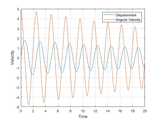
1. Graph for the velocity v/s time which shows Displacement and Angular velocity

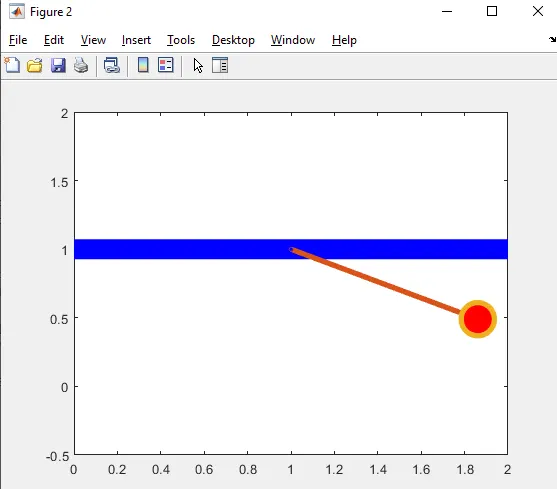
2. Animation of the pendulum plotted.

Snapshot:

Google Drive LInk

The animated video is uploaded in Google Drive with open access. The Google drive link is shared below:-

https://drive.google.com/file/d/11S-ULfna46PnkMvJywlRGuiQroOzP8mn/view?usp=sharing

CONCLUSION :

1. We have successfully plotted the graph of Displacement Angular Velocity in Velocity v/s Time diagram.
2. We have successfully created a movie of animation of a Simple Pendulum in Operation with all of the parameters.

ERRORS :

• While using marker command inside the for loop for animation of Simple Pendulum, i have used '0' instead of 'O', to mark the Pendulum Bob.
• as, the MATLAB, is case-sensitive, an error is thrown as "Invalid color or line style".

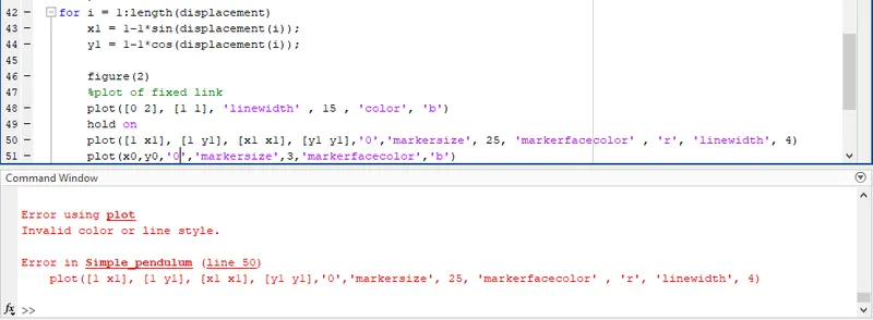
• So, i just replaced 'O', instead of '0', to overcome this Error and the program run thoroughly and successfully.