Project 2 - Rankine cycle Simulator
AIM :
To create a Rankine Cycle Simulator using MATLAB.
- Calculate each state points of the Rankine Cycle (any type of your choice) based on user inputs.
- Plot the corresponding T-s and h-s plots for the given set of inputs.
- Calculate Efficiency.
The Rankine cycle is an idealized thermodynamic cycle of a heat engine that converts heat into mechanical work while undergoing a phase change. It is an idealized cycle in which friction losses in each of the four components are neglected. The heat is supplied externally to a closed loop, which usually uses water as the working fluid.
- Four components of the Rankine cycle:
- Four processes of the Rankine cycle:
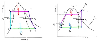
- The difference between Turbine work and compressor work is known as Net work output.
`W_n = W_T - W_P`
Back-Work Ratio
- Ratio of Compressor work to the Turbine work is known as Back-Work Ratio.
`R_(BW)=W_P/W_T`
- The efficiency of the Steam Cycle is given by,
`eta =W_n/Q_1 = (W_T-W_P)/Q_1`
- Applying the Steady Flow Energy Equation (SFEE) to all the process, neglecting the Friction losses and changs in Kinetic & Potential Energy,
- Q1-hi-h4 (Boiler)
- Wt=hl-h2 (Turbine)
- Q2=h2-h3 (Condenser)
- Wp=h4-h3 (Pump)
- The Capacity of the Steam Plant is often expressed interms of Steam Rate (SR) or Specific Steam Consumption (SSC)
- One file, named as 'XSteam', has been provided.
- we have to download the file, and save it in the same folder in which the current matlab program exists.
- The file provided, is also a MATLAB file, containing different values similar to our Steam Table, which will be helpful for our programming, which we can call as a function.
2. Represent the processes in Command Window
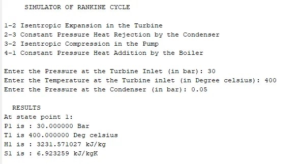
- As a specific pattern of Output is demanded in Command Window, we have to present the different Processes, in a Rankine Cycle, as follows:
fprintf('     SIMULATOR OF RANKINE CYCLE \n\n')
fprintf('1-2 Isentropic Expansion in the Turbine\n')
fprintf('2-3 Constant Pressure Heat Rejection by the Condenser \n')
fprintf('3-2 Isentropic Compression in the Pump \n')
fprintf('4-1 Constant Pressure Heat Addition by the Boiler \n\n')
3. Code to ask user inputs:
- As it is asked to create the program, to take user inputs for calculations, we will use input command, which will enable us to provide values during program running.
%inputs

P1 =input('Enter the Pressure at the Turbine Inlet (in bar): ');
T1 = input('Enter the Temperature at the Turbine inlet (in Degree celsius): ');
P2=input('Enter the Pressure at the Condenser (in bar): ');
fprintf('\n')
disp('  RESULTS')
4. Getting different values from 'XSteam' file
The most important part of our programming is calculation, for which we need different values such as
- CpV_p (Saturated vapour heat capacity)
- CvV_p (Saturated vapour isochoric heat capacity)
- CpL_p (Saturated liquid heat capacity)
- CvL_p (Saturated liquid isochoric heat capacity)
- Tsat_p (Saturation temperature)
- sV_p (Saturated vapour entropy)
- sL_p (Saturated liquid entropy)
- hL_p (Saturated liquid enthalpy)
- hV_p (Saturated vapour enthalpy)
And we can get the above values from XSteam file provided.
%getting Cp and Cv values from Xsteam
%Cp and Cv assumed to not change with temperature for simplicity

% for vapour
high_cpV= XSteam ('CpV_p', P1);
low_cpV=XSteam ( 'CpV_p', P2);
high_cvV=XSteam ('CvV_P', P1);
low_cvV=XSteam ( 'CvV_p', P2);

% for liquid
high_cpL= XSteam ('CpL_p', P1);
low_cpL= XSteam ('CpL_p', P2);
high_cvL=XSteam ('CvL_p', P1);
low_cvL=XSteam ('CvL_p', P2);

%Getting important parameters from Xsteam
%for high pressure

T1s = XSteam ('Tsat_p', P1);
S1g = XSteam('sV_p', P1);
S1f = XSteam('SL_p', P1);
S1fg = S1g - S1f;
H1f= XSteam ('hL_p', P1);
H1g =XSteam('hV_p', P1);
H1fg = H1g - H1f;

%for low pressure

T2s =XSteam('Tsat_p', P2);
S2g = XSteam('sV_p', P2);
S2f= XSteam( 'SL_p', P2);
S2fg = S2g - S2f;
H2f = XSteam ('hL_p', P2);
H2g = XSteam('hV_p', P2);
H2fg = H2g - H2f;
5. Define State point values
- We need to define the values for the four State points.
- the values we need, is available in XSteam file.
%% State point 1
disp('At state point 1:')

fprintf('P1 is : %f Bar \n', P1)
fprintf('T1 is %f Deg celsius \n', T1)

H1 = XSteam('h_pt', P1, T1);

fprintf('H1 is : %f kJ/kg \n', H1)

S1 = XSteam('s_pt', P1, T1);

fprintf('S1 is : %f kJ/kgK \n\n', S1)

%% State point 2
disp('At state point 2:')
fprintf('P2 is: %f Bar \n', P2)         %P2 input already taken

S2 = S1;
fprintf('S2 is: %f kJ/kgK \n', S2)

%predicting location of point 2 in T-s
if(S2<=S2g)
    X2= (S2- S2f) / (S2fg);            % Dryness fraction at state point 2
else
    X2=1;
end
fprintf('X2 is :%f \n', X2)

%calculating T2 for superheat or wet or dry wherever it lies

if(X2<1)
    T2=T2s;
else
    %t2 cal by s2 s2g+low_cpV* (log(T2/T2s)
    T2=(T2s+273.15)*exp((S2-S2g)/low_cpV); %2 in superheated region
    T2=T2-273.15;
end
fprintf('T2 is: %f Deg celsius \n', T2)

if (X2<1)
    H2=H2f+ X2 * H2fg;
else
    H2=H2g+ low_cpV* (T2-T2s);
end
fprintf('H2 is: %f kJ/kg \n\n', H2)

%% State point 3
%Assuming no subcooling in condensor
disp('At state point 3:')

P3 = P2;
fprintf('P3 is %f Bar \n', P3)
V3 =XSteam('vL_p', P3);

T3 = T2s;                          %no subcooling assumed
fprintf('T3 is: %f Deg celsius \n', T3)

H3 =H2f;
fprintf('H3 is: %f kJ/kg \n', H3)

S3 =S2f;
fprintf('S3 is: %f kJ/kgK \n\n', S3)

%% State point 4
disp('At state point 4:')
P4 = P1;
fprintf('P4 is: %f Bar \n', P4)

S4 = S3;
fprintf('S4 is %f kJ/kgK \n', 54)
6. Calculations
- we have to use different formulas to get required values which will be used in calculation of Output values.
%% calculations
%Compressor Work
Wp = V3* (P4 - P3)* 100;
H4 =Wp + H3;
fprintf('H4 is %f kJ/kg \n', H4)

%Turbine Work
Wt= H1 -H2;

% to cal T4 s4-s3-sf1-high_cpl*ln(t1s/t4)
term=exp((S1f-S4)/high_cpL);                    %Use exp instead of Exp to take input as doubles
T4= T1s/term;
fprintf('T4 is: %f Deg celsius \n\n', T4)

fprintf('Work by turbine is : %f kJ/kg \n',Wt)
fprintf('Work by compressor is %f kJ/kg \n', Wp)

%Heat input
Qin= H1- H4;
7. Calculation of Required Outputs
%%Outputs Required
%Net work Output
Wnet =Wt- Wp;
fprintf('Net Work Output is : %f kJ/kg \n', Wnet)

%Back-Work Ratio
R_BW=Wp/Wt;
fprintf('Back-Work Ratio is : %f\n', R_BW)

%Thermal Efficiency
eff_thermal = (Wnet / Qin);
fprintf('Thermal efficiency is: %f', eff_thermal*100); disp('%')

%Steam Rate or Specific steam consumption
SSC = 3600 / Wt;
fprintf('S.S.C is : %f kg/kWh ', SSC)
8. Calculation for plotting Liquid and Vapour lines
- Here, we will use linspace for different values of temp.
- temp will be used in for-loop.
- for-loop, is used for getting different values for Entropy(H_L, H_v) and Enthalpy(S_L, S_V)
- we get values for (H_L, H_v) and (S_L, S_V), from XSteam file.
%% Calculation for plotting Liquid and Vapour lines

temp = linspace(1, 373, 500);
for i=1: length (temp)
    H_L(i)= XSteam('hL_T', temp(i));
    H_V(i)= XSteam('hV_T', temp(i));
    S_L(i)= XSteam('sL_T', temp(i));
    S_V(i)= XSteam('sV_T', temp(i));
end
9. Plotting T-S and H-S Diagrams
- Here, we use different parameters, which need to be holded, so the hold on command in plotting is used.
- As Output of the plots are required in specific order, so we have to replace all of the coordinate values to point names, such as:
for T-S diagram
- (S1, T1) - '1'
- (S2, T2) - '2'
- (S2g, T2s) - '2s'
- (S3, T3) - '3'
- (S4, T4) - '4'
- (S1f, T1s) - '4s'
- (S1g, T1s) - '1s'
for H-S diagram
- (S1, H1) - '1'
- (S2, H2) - '2'
- (S3, H3) - '3'
- (S4, H4) - '4'
To replace all these values we will use text command
%% Plotting T-S and H-S Diagrams
%For T-S diagram
figure (1)
hold on
plot([S1 S2], [T1 T2], 'r', 'linewidth', 1)
text(S1, T1, ' 1')
text(S2, T2, ' 2')
plot([S2 S2g], [T2 T2s], 'r', 'linewidth',1)
text (S2g, T2s,' 2s')
plot([S2g S3], [T2s T3], 'r', 'linewidth',1)
text (S3, T3, ' 3')
plot([S3 S4], [T3 T4], 'r', 'linewidth', 1)
text (S4, T4,' 4')
plot([S4 S1f], [T4 T1s], 'r', 'linewidth',1)
text (S1f, T1s,' 4s')
plot([S1f S1g], [T1s T1s], 'r', 'linewidth',1)
text (S1g, T1s, '1s')
plot([S1g S1], [T1s T1], 'r', 'linewidth',1)
plot (S_L, temp, 'b', 'linestyle', '-' ,'linewidth',1)
plot (S_V, temp, 'b', 'linestyle', '-','linewidth',1)


title('T-S Diagram of Ideal Rankine Cylce')
ylabel('Temprature (degC)')
xlabel('Specific Entropy (kJ/kgK)')

%For H-S diagram
figure(2)
hold on
plot([S1 S2], [H1 H2], 'r', 'linewidth', 1);
text (S1, H1,' 1')
plot([S2 S3], [H2 H3], 'r', 'linewidth', 1);
text (S2, H2,' 2')
plot([S3 S4], [H3 H4], 'r', 'linewidth', 1);
text (S3, H3,' 3')
plot([S4 S1], [H4 H1], 'r', 'linewidth', 1);
text (S4, H4,' 4')
plot (S_L, H_L, 'b','LineWidth',0.5)
plot (S_V, H_V, 'b','LineWidth',0.5)

title('H-S Diagram of Ideal Rankiete Cylce')
ylabel('Specific Enthalpy (kJ/kg)')
xlabel('Specific Entropy (kJ/kgK)')
MAIN PROGRAMMING :
clear all
close all
clc

fprintf('     SIMULATOR OF RANKINE CYCLE \n\n')
fprintf('1-2 Isentropic Expansion in the Turbine\n')
fprintf('2-3 Constant Pressure Heat Rejection by the Condenser \n')
fprintf('3-2 Isentropic Compression in the Pump \n')
fprintf('4-1 Constant Pressure Heat Addition by the Boiler \n\n')

%inputs

P1 =input('Enter the Pressure at the Turbine Inlet (in bar): ');
T1 = input('Enter the Temperature at the Turbine inlet (in Degree celsius): ');
P2=input('Enter the Pressure at the Condenser (in bar): ');
fprintf('\n')
disp('  RESULTS')

%getting Cp and Cv values from Xsteam
%Cp and Cv assumed to not change with temperature for simplicity

% for vapour
high_cpV= XSteam ('CpV_p', P1);
low_cpV=XSteam ( 'CpV_p', P2);
high_cvV=XSteam ('CvV_P', P1);
low_cvV=XSteam ( 'CvV_p', P2);

% for liquid
high_cpL= XSteam ('CpL_p', P1);
low_cpL= XSteam ('CpL_p', P2);
high_cvL=XSteam ('CvL_p', P1);
low_cvL=XSteam ('CvL_p', P2);

%Getting important parameters from Xsteam
%for high pressure

T1s = XSteam ('Tsat_p', P1);
S1g = XSteam('sV_p', P1);
S1f = XSteam('SL_p', P1);
S1fg = S1g - S1f;
H1f= XSteam ('hL_p', P1);
H1g =XSteam('hV_p', P1);
H1fg = H1g - H1f;

%for low pressure

T2s =XSteam('Tsat_p', P2);
S2g = XSteam('sV_p', P2);
S2f= XSteam( 'SL_p', P2);
S2fg = S2g - S2f;
H2f = XSteam ('hL_p', P2);
H2g = XSteam('hV_p', P2);
H2fg = H2g - H2f;

%% State point 1
disp('At state point 1:')

fprintf('P1 is : %f Bar \n', P1)
fprintf('T1 is %f Deg celsius \n', T1)

H1 = XSteam('h_pt', P1, T1);

fprintf('H1 is : %f kJ/kg \n', H1)

S1 = XSteam('s_pt', P1, T1);

fprintf('S1 is : %f kJ/kgK \n\n', S1)

%% State point 2
disp('At state point 2:')
fprintf('P2 is: %f Bar \n', P2)         %P2 input already taken

S2 = S1;
fprintf('S2 is: %f kJ/kgK \n', S2)

%predicting location of point 2 in T-s
if(S2<=S2g)
    X2= (S2- S2f) / (S2fg);            % Dryness fraction at state point 2
else
    X2=1;
end
fprintf('X2 is :%f \n', X2)

%calculating T2 for superheat or wet or dry wherever it lies

if(X2<1)
    T2=T2s;
else
    %t2 cal by s2 s2g+low_cpV* (log(T2/T2s)
    T2=(T2s+273.15)*exp((S2-S2g)/low_cpV); %2 in superheated region
    T2=T2-273.15;
end
fprintf('T2 is: %f Deg celsius \n', T2)

if (X2<1)
    H2=H2f+ X2 * H2fg;
else
    H2=H2g+ low_cpV* (T2-T2s);
end
fprintf('H2 is: %f kJ/kg \n\n', H2)

%% State point 3
%Assuming no subcooling in condensor
disp('At state point 3:')

P3 = P2;
fprintf('P3 is %f Bar \n', P3)
V3 =XSteam('vL_p', P3);

T3 = T2s;                          %no subcooling assumed
fprintf('T3 is: %f Deg celsius \n', T3)

H3 =H2f;
fprintf('H3 is: %f kJ/kg \n', H3)

S3 =S2f;
fprintf('S3 is: %f kJ/kgK \n\n', S3)

%% State point 4
disp('At state point 4:')
P4 = P1;
fprintf('P4 is: %f Bar \n', P4)

S4 = S3;
fprintf('S4 is %f kJ/kgK \n', 54)

%% calculations
%Compressor Work
Wp = V3* (P4 - P3)* 100;
H4 =Wp + H3;
fprintf('H4 is %f kJ/kg \n', H4)

%Turbine Work
Wt= H1 -H2;

% to cal T4 s4-s3-sf1-high_cpl*ln(t1s/t4)
term=exp((S1f-S4)/high_cpL);                    %Use exp instead of Exp to take input as doubles
T4= T1s/term;
fprintf('T4 is: %f Deg celsius \n\n', T4)

fprintf('Work by turbine is : %f kJ/kg \n',Wt)
fprintf('Work by compressor is %f kJ/kg \n', Wp)

%Heat input
Qin= H1- H4;

%%Outputs Required
%Net work Output
Wnet =Wt- Wp;
fprintf('Net Work Output is : %f kJ/kg \n', Wnet)

%Back-Work Ratio
R_BW=Wp/Wt;
fprintf('Back-Work Ratio is : %f\n', R_BW)

%Thermal Efficiency
eff_thermal = (Wnet / Qin);
fprintf('Thermal efficiency is: %f', eff_thermal*100); disp('%')

%Steam Rate or Specific steam consumption
SSC = 3600 / Wt;
fprintf('S.S.C is : %f kg/kWh ', SSC)

%% Calculation for plotting Liquid and Vapour lines

temp = linspace(1, 373, 500);
for i=1: length (temp)
    H_L(i)= XSteam('hL_T', temp(i));
    H_V(i)= XSteam('hV_T', temp(i));
    S_L(i)= XSteam('sL_T', temp(i));
    S_V(i)= XSteam('sV_T', temp(i));
end

%% Plotting T-S and H-S Diagrams
%For T-S diagram
figure (1)
hold on
plot([S1 S2], [T1 T2], 'r', 'linewidth', 1)
text(S1, T1, ' 1')
text(S2, T2, ' 2')
plot([S2 S2g], [T2 T2s], 'r', 'linewidth',1)
text (S2g, T2s,' 2s')
plot([S2g S3], [T2s T3], 'r', 'linewidth',1)
text (S3, T3, ' 3')
plot([S3 S4], [T3 T4], 'r', 'linewidth', 1)
text (S4, T4,' 4')
plot([S4 S1f], [T4 T1s], 'r', 'linewidth',1)
text (S1f, T1s,' 4s')
plot([S1f S1g], [T1s T1s], 'r', 'linewidth',1)
text (S1g, T1s, '1s')
plot([S1g S1], [T1s T1], 'r', 'linewidth',1)
plot (S_L, temp, 'b', 'linestyle', '-' ,'linewidth',1)
plot (S_V, temp, 'b', 'linestyle', '-','linewidth',1)


title('T-S Diagram of Ideal Rankine Cylce')
ylabel('Temprature (degC)')
xlabel('Specific Entropy (kJ/kgK)')

%For H-S diagram
figure(2)
hold on
plot([S1 S2], [H1 H2], 'r', 'linewidth', 1);
text (S1, H1,' 1')
plot([S2 S3], [H2 H3], 'r', 'linewidth', 1);
text (S2, H2,' 2')
plot([S3 S4], [H3 H4], 'r', 'linewidth', 1);
text (S3, H3,' 3')
plot([S4 S1], [H4 H1], 'r', 'linewidth', 1);
text (S4, H4,' 4')
plot (S_L, H_L, 'b','LineWidth',0.5)
plot (S_V, H_V, 'b','LineWidth',0.5)

title('H-S Diagram of Ideal Rankiete Cylce')
ylabel('Specific Enthalpy (kJ/kg)')
xlabel('Specific Entropy (kJ/kgK)')
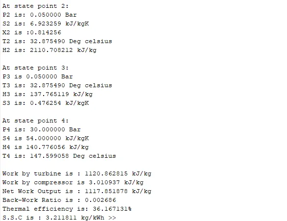
OUTPUTS :
- Plottings
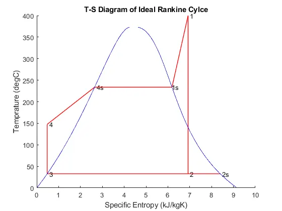
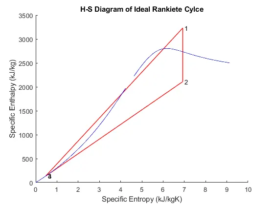
- Screenshot of Command Window
ERRORS :
- Fortunately during this program, no Error is encountered throughout the program.
CONCLUSION :
- Program for Rankine cycle simulator in MATLAB is successfully executed
- Different functions and commands learned.