Air Standard Cycle
AIM :
To write a MATLAB program to solve an Otto cycle, and make plots for it.
OBJECTIVES :
- To Plot the P-V Diagram of an Otto Cycle.
- To find the Thermal Efficiency of the Otto Cycle.
INTRODUCTION :
An Otto cycle is an idealized Thermodynamic Cycle that describes the functioning of a typical spark ignition piston Engine. It is the thermodynamic cycle most commonly found in automobile engines, which is also known as Petrol Engine.
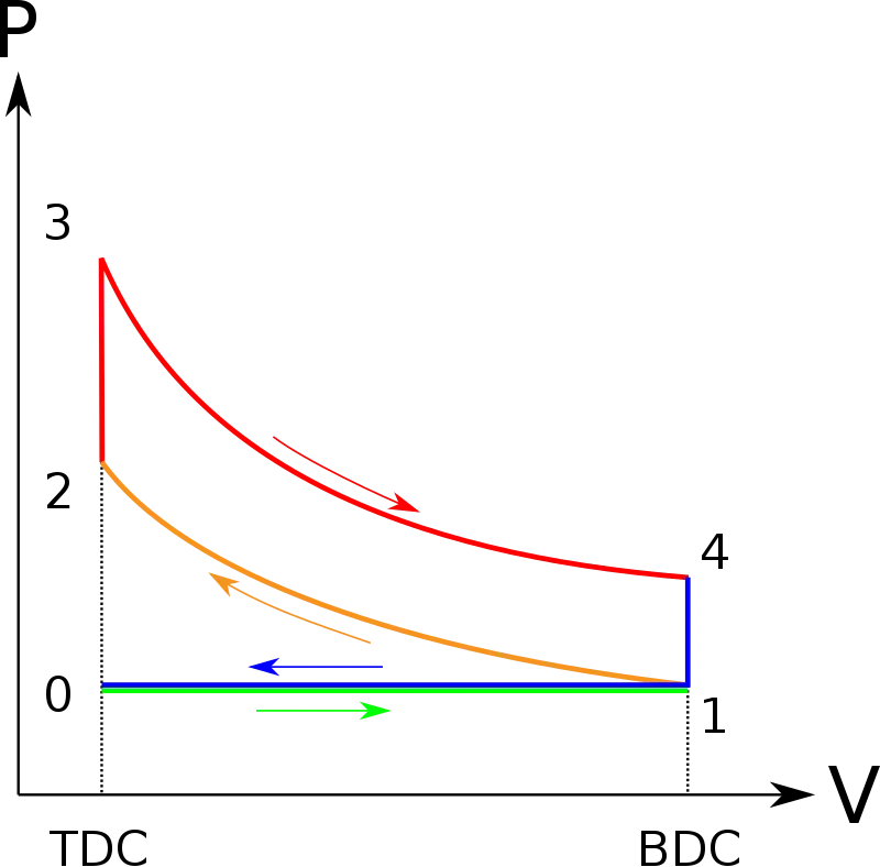
Process of an Otto Cycle engine as follows:-
- Suction stroke - Process (0`to`1), intakes fuel.
- Compression stroke - Process (1`to`2), Isentropic compression of fuel.
- Combustion stroke - Process (2`to`3), isochoric combustion of fuel or heat addition.
- Power stroke - Process (3`to`4), Isentropic expansion of fuel.
- Exhaust stroke - Process (4`to`1), isochoric exhaustion of fuel or heat rejection.
PISTON KINEMATICS
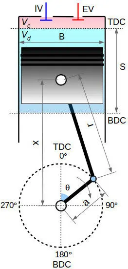
Piston Kinematics consists of some main parameters such as:
- Bore
- Stroke
- Connecting Rod
- Compression Ratio
Equations used in Piston Kinematics:
- `(V_1)/(V_c) = 1+(R_c-1)[R+1-costheta-root2(R^2-sin^2theta)]`
Where,
`Rc` = Compression ratio
`R` = Ratio of Connecting rod length to Crank
Thermal Efficiency:
`eta_o = 1-1/(R_c^(gamma-1))`
Some Other Equations used:
- Isentropic Compression & power`=> P*V^(gamma) = Constant`
- Isochoric heat addition and rejection`=> P/T= Constant`
- Ideal Gas Equation `=> (P*V)/T = Constant`
- Compression Ratio `=> (V_s +V_c) /V_c`
STEPS AND PROCEDURES :
STEP-1 : Defining input Parameters
- First of all, we need to define the input parameters
%%inputs

%Adiabatic Constant
gamma = 1.4;

%%Engine geometric Parameters

%Bore diameter (m)
Bore = 0.094;
%Stroke Length (m)
Stroke = 0.082;
%Connecting Rod length (m)
Con_Rod = 0.585;
%Compression Ratio
CR = 12;
Then, we need to define the State 1 parameters
%%State variables at state point 1
%Pressure at the start of Compression (Pa)
P1 = 101325;
%Temperature at the start of compression (K)
T1 = 320;
%%Calculating the swept volume and the clearance volume
%Volume swept by the piston (m^3)
V_swept = (pi/4)*Bore^2*Stroke;
%CLearance Volume
V_clearance = V_swept/(CR-1);
%Volume at the start of compression
V1 = V_swept + V_clearance;- Then, the step 2 parameters should be defined
%State variables at state point 2
%P2V2^gamma = P1V1^gamma
%P2 = P1*(V1/V2)^gamma; => P2 = P1*CR^gamma
P2 = P1*CR^gamma;
V2 = V_clearance;
%P1V1/T1 = P2V2/T2 => T2 = P2*V2*T1/(P1*V1)
T2 = P2*V2*T1/(P1*V1);- As the next step, we shoud define the State 3 parameters,
%state variables at state point 3
%P3V3/T3 = P2V2/T2 => P3 = P2*T3/T2
P3 = P2*T3/T2;
V3 = V2;
T3 = 2000- As the above 3 state parameters, State 4 parameters should be defined,
%STATE VARIABLES at state point 4
V4 = V1;
%P3V3^gamma P4V4^gamma => P4 = P3(V3/V4)^gamma
P4 = P3*(V3/V4)^gamma;
T4 = (P4*V4*T3)/(P3*V3)
STEP-2 : Writing code for Plotting points
- we have to write a code to have the above input parameters, plotted as points.
%%Plotting
figure(1)                           %Create Figure window
hold on                             %Retain current plots when adding new plots
plot(V1,P1,'*', 'color', 'r')       %To plot State 1 values
plot(V2,P2,'*', 'color', 'r')       %To plot State 2 values
plot(V3,P3,'*', 'color', 'r')       %To plot State 3 values
plot(V4,P4,'*', 'color', 'r')       %To plot State 4 values
xlabel('Volume (m^3)')              %Label for X-Axis
ylabel('Pressure (Pa)')             %Label for Y-Axis
grid on %Display grid lines- Now, the output for the above code is as below:
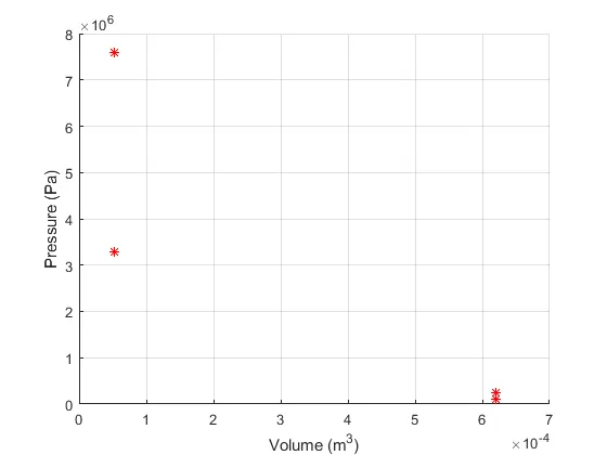
- Here, we can observe that, we only got the points plotted, but further we need to plot the curves too. For those curves, we need to find out the Instantaneous pressure and volume as the Piston operates.
- And to find out these instantaenous points, we have to define a function as discussed in further steps.
STEP-3 : Defining Function
- To find out the instantaenous points, we have to define a function "air_standard_cycle" to an array named "[V]".
- Here, in this Function, we have to pass the input parameters, in order to calculate instantaneous points.
function [V] = air_standard_cycle(Bore,Stroke,Con_Rod,CR,Start_Crank,End_Crank)

%Engine geometric Parameters

a = Stroke/2
R=Con_Rod/a


%Calculating the swept volume and the clearance volume
V_swept = (pi/4)*Bore^2*Stroke
V_clearance = V_swept/(CR-1)

theta = linspace(Start_Crank,End_Crank,100);

term1 = 0.5*(CR-1);
term2 = R+1 - cosd(theta);
term3 = (R^2 - sind(theta).^2).^0.5;

V = (1+term1*(term2-term3)).*V_clearance;


end- The above Function, is created only to plot isentropic process curve.
- In next step, we would call this function inside our main program.
STEP-4 : Calling Function
- So, this function is only called in between the primary programming below the Isentropic Compression and Isentropic Expansion, i.e., under State 2 and State 3 values, respectively, as below:-
%State variables at state point 2

%P2V2^gamma = P1V1^gamma
%P2 = P1*(V1/V2)^gamma; => P2 = P1*CR^gamma
P2 = P1*CR^gamma;
V2 = V_clearance;
%P1V1/T1 = P2V2/T2 => T2 = P2*V2*T1/(P1*V1)
T2 = P2*V2*T1/(P1*V1);

%Calling function to plot the isentropic curve
V_compression = air_standard_cycle(Bore,Stroke,Con_Rod,CR,180,0);
constant_C = P1*V1^gamma;
P_compression = constant_C./V_compression.^gamma;

%state variables at state point 3
%P3V3/T3 = P2V2/T2 => P3 = P2*T3/T2
P3 = P2*T3/T2;
V3 = V2;
T3 = 2000


%Calling function to plot the isentropic curve
V_expansion = air_standard_cycle(Bore,Stroke,Con_Rod,CR,0,180);
constant_C = P3*V3^gamma;
P_expansion = constant_C./V_expansion.^gamma;- Now, the instantaneous points for the isentropic curve is calculated by this function. But we need to plot the curve, as next step.
STEP-5 : Plotting the Curves
- Earlier, we have plotted points, now we need to joint the points by plotting curves as follows:
plot(V_compression, P_compression)  %To plot isentropic curve for State 1 to State 2
plot([V2 V3],[P2 P3],'color', 'b')  %To plot Isochoric curve for State 2 to State 3
plot(V_expansion, P_expansion)      %To plot isentropic curve for State 3 to State 4
plot([V4 V1],[P4 P1],'color', 'b')  %To plot Isochoric curve for State 4 to State 1
STEP-6 : Write code for Thermal Efficiency
%Thermal Efficiency of this Otto Cycle
 etta_otto = 1-(1/((CR^(gamma-1))));
%Thermal Efficiency Percentage
etta_otto = etta_otto*100;
Therma_Efficiency_percentage = etta_otto
PROGRAMMING :
- Here, we will look at the total programming as we have written in step by step above and execute the same to ge the output as P-V diagram of an Otto Cycle engine.
clear all
close all
clc

%%inputs

%Adiabatic Constant
gamma = 1.4;
T3 = 2000;

%%Engine geometric Parameters

%Bore diameter (m)
Bore = 0.094;
%Stroke Length (m)
Stroke = 0.082;
%Connecting Rod length (m)
Con_Rod = 0.585;
%Compression Ratio
CR = 12;

%%State variables at state point 1

%Pressure at the start of Compression (Pa)
P1 = 101325;
%Temperature at the start of compression (K)
T1 = 320;

%%Calculating the swept volume and the clearance volume

%Volume swept by the piston (m^3)
V_swept = (pi/4)*Bore^2*Stroke;
%CLearance Volume
V_clearance = V_swept/(CR-1);
%Volume at the start of compression
V1 = V_swept + V_clearance;


%State variables at state point 2
%P2V2^gamma = P1V1^gamma
%P2 = P1*(V1/V2)^gamma; => P2 = P1*CR^gamma
P2 = P1*CR^gamma;
V2 = V_clearance;
%P1V1/T1 = P2V2/T2 => T2 = P2*V2*T1/(P1*V1)
T2 = P2*V2*T1/(P1*V1);

%Calling function to plot the isentropic curve
V_compression = air_standard_cycle(Bore,Stroke,Con_Rod,CR,180,0);
constant_C = P1*V1^gamma;
P_compression = constant_C./V_compression.^gamma;

%state variables at state point 3
%P3V3/T3 = P2V2/T2 => P3 = P2*T3/T2
P3 = P2*T3/T2;
V3 = V2;
T3 = 2000

%Calling function to plot the isentropic curve
V_expansion = air_standard_cycle(Bore,Stroke,Con_Rod,CR,0,180);
constant_C = P3*V3^gamma;
P_expansion = constant_C./V_expansion.^gamma;


%STATE VARIABLES at state point 4
V4 = V1;

%P3V3^gamma P4V4^gamma => P4 = P3(V3/V4)^gamma
P4 = P3*(V3/V4)^gamma;
T4 = (P4*V4*T3)/(P3*V3)

%%Plotting
figure(1)                           %Create Figure window
hold on                             %Retain current plots when adding new plots

plot(V1,P1,'*', 'color', 'r')       %To plot State 1 values
plot(V_compression, P_compression)  %To plot isentropic curve for State 1 to State 2
plot(V2,P2,'*', 'color', 'g')       %To plot State 2 values
plot([V2 V3],[P2 P3],'color', 'cyan')  %To plot Isochoric curve for State 2 to State 3
plot(V3,P3,'*', 'color', 'b')       %To plot State 3 values
plot(V_expansion, P_expansion)      %To plot isentropic curve for State 3 to State 4
plot(V4,P4,'*', 'color', 'y')       %To plot State 4 values
plot([V4 V1],[P4 P1],'color', 'magenta')  %To plot Isochoric curve for State 4 to State 1

xlabel('Volume (m^3)')              %Label for X-Axis
ylabel('Pressure (Pa)')             %Label for Y-Axis
legend("Initial State","Isentropic Compression", "State prior to heat addition","Isochoric Heat Addition", "State prior to Expansion", "Isentropic Expansion", "State prior to Heat Rejection", "Isochoric Heat rejection") %labelling points and curves inside the plots
title("OTTO CYCLE")                 %Labelling the plot title
grid on                             %Display grid lines

%Thermal Efficiency of this Otto Cycle
 etta_otto = 1-(1/((CR^(gamma-1))));
%Thermal Efficiency Percentage
etta_otto = etta_otto*100;
Therma_Efficiency_percentage = etta_otto
OUTPUT :
Plot of P-V diagram of an Otto cycle
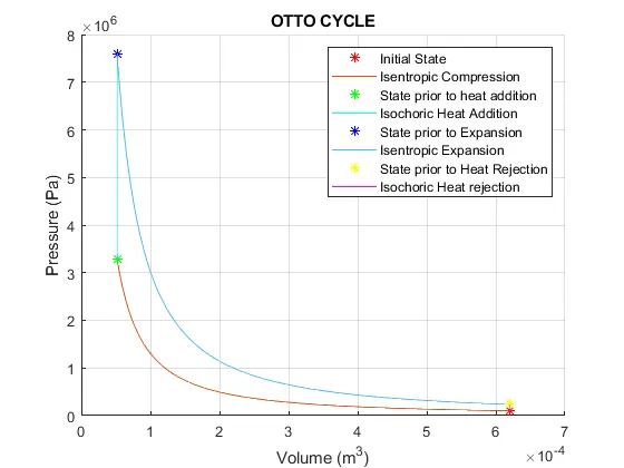
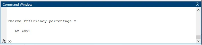
Thermal Efficiency
CONCLUSION :
- The above program for simulation of P-V Diagram of an Otto cycle, is successfully compiled and Executed.
- We also get the Thermal Efficiency of this Otto Cycle as 62.98% (approximately).
ERROR :
- When saving and running the program in which i defined the function "air_standard_cycle", i have not noticed that, this program is not been saved to the same disk, where my main program was saved, so for that reason, the error thrown is as follows:
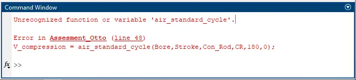
- So to overcome this error, i just changed the path of program files, so both of the program files saved in the same path.
- Then, it run successfully.