Week 3 - Solving second order ODEs

Aim- write the program to solve second order ODE using Matlab and aminate the oscillation of the simple pendulum.

ODE= order differential equation.

ODE is the extremely l important in engineering the describe a lot of important finominal and solving these ODEs can actually help us understand the systems

this equation is derived to solve the second-order ODE

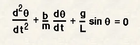
where-

theta=angular displacement

b=damping coiefficient

l=length of connecting string

t=osilating time

m= mass

g= gravity

writing function command program

Function command is nothing but a piece of code that we can reuse by just calling its name and passing in the right parameters.

writing of function code

function [dtheta_dt]= ode_func(t,theta,b,m,g,l)

theta1 = theta(1)
theta2 = theta(2)
dtheta1_dt = theta2
dtheta2_dt = -(b/m)*theta2-(g/l)*sin(theta1)
dtheta_dt = [dtheta1_dt;dtheta2_dt]
end

coding

• at first, we have to use the word Function to start the function command
• and then we want to create a templet and this is a code templet and name for the templet
• we are going to name the code templet as ode_function
• we are going to use this equation to solve the ode equation.

• so whenever we want to substitute different values we just call this function and then pass in the right values
• then we have to save the function while saving the name of the function and the name of the file should exactly be the same
• the calling the function means using the function and using the templates with the appropriate values
• we have to ensure the no of inputs we provide match the orders of inputs also match
• and this equation is very large so we are going to break it up into several terms.
• end word id is used to end the function command.

Inputs

l=1

m=1

b=0.05

g=9.81

t=0to20

angular displacement=0

angular velocity=3 rad/sec

writing the main code

%solving the second order ODE
close all
clear all
clc

%inputs
l=1
m=1
b=0.05
g=9.81

%initial conditions
theta_0=[0;3];

%time points
t_span=linspace(0,20,500);

%solving of the ODE
[t,results]=ode45(@(t,theta)ode_func(t,theta,b,m,g,l),t_span,theta_0)

figure(1)
plot(t,results(:,1))
hold on
plot(t,results(:,2))
ylabel('plot')
xlabel('time')

ct=1
for i=1:length(results(:,1));
    x0=0
    y0=0
    y1=-1*cos(results(i));
    x1=1*sin(results(i));

%plotting
figure(2)
plot([-1 1],[0 0],'linewidth',3,'Color','b')
hold on
plot([x0 x1],[y0 y1],'LineWidth',2,'Color','y')
plot(x1,y1,'marker','o','Markersize',25,'Markerfacecolor','r')
axis([-1.5 1.5 -1.5 0.5])
M(ct) = getframe(gcf);
ct=ct+1
hold off
end


movie(M)
videofile=VideoWriter('ode_challenge.avi','uncompressed avi')
open(videofile)
writeVideo(videofile,M)
close(videofile)

• to get started we have to open a new file
• whenever we start a new program it is good practice to include some commands
• input variables are taken
• we have to ensure the no of inputs we provide match the orders of inputs also match
• we have to ensure that both the function program and the working program must be in the same folder
• and then we have to calculate the required values after calculating the required values
• we have to use the plot command to create a graph

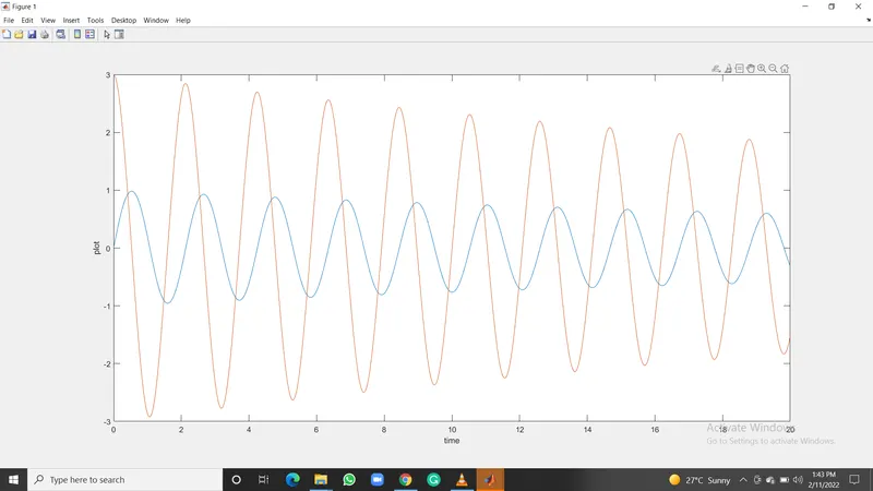
output

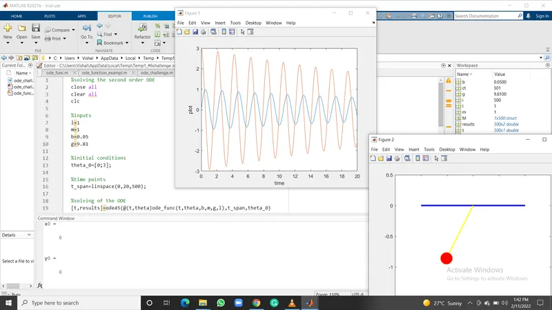
graph

Animated video

oscillation of the pendulum

error faced during the animating video

error link