Week 3 - Solving second order ODEs

Aim:

Write a program in Matlab\Octave that will simulate the pendulum motion.

Requirements:

• For each value in time
• Create an image that represents the position of the pendulum
• You can assume the length of the string and the size of the ball
• Use the marker command to create a sphere
• One end of the pendulum is fixed
• The other end moves according to the solution of the ODE you had solved.
• If you are using using Matlab, use the movie command create an animation
• If you are using Octave you need to generate images first and then stitch them to form the animation
• Upload an animation on You tube and provide the You tube link for an animation in your report.

Basic Information On Simple Pendulum:

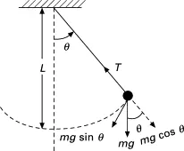
The simple pendulum is another mechanical system that moves in an oscillatory motion. It consists of a point mass 'm' suspended by means of light inextensible string of length L from a fixed support . The motion occurs in a vertical plane and is driven by a gravitational force. As Shown in fig.below:

Governing Equation:

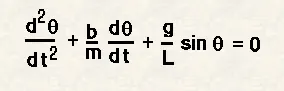
This Second order of ODE represents the equation of motion of a simple pendulum .

In the above equation,

g = gravity in m/s2,

L = length of the pendulum in m,

m = mass of the ball in kg,

b=damping coefficient.

Parameters Given:

L=1 metre,

m=1 kg,

b=0.05.

g=9.81 m/s2.

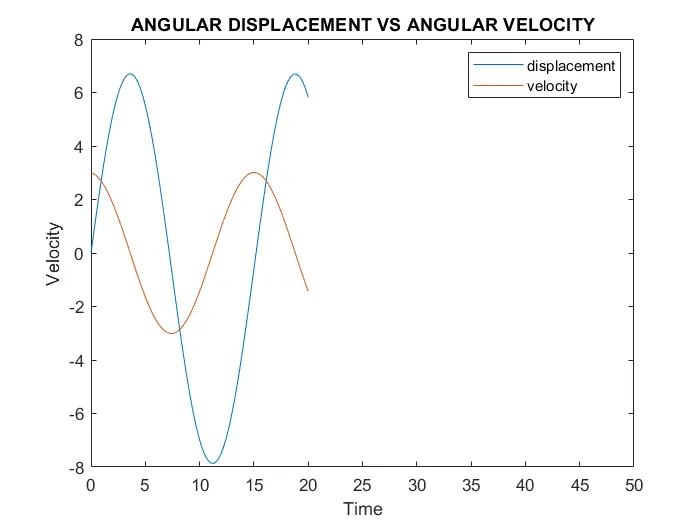
Simulate the motion between 0-20 sec, for angular displacement=0,angular velocity=3 rad/sec at time t=0.

Matlab Program:

clear all
close all
clc

%input
b=0.05;
g=9.81;
l=1;
m=1;

% initial condition
initial = [0;3];

% time points
time=linspace(0,20,500);

% solve ode 
[t,results] = ode45(@(t,theta) ode_func(t, theta, b,g,l,m),time,initial);

% plot
C=1;

for i=1:length(results(:,1))

    x1 = -l*sind(results(i,1))
    y1 = -l*cosd(results(i,1))
   

    
    plot([0,x1],[0,y1],'LineWidth',1);
    hold on
    plot(x1,y1,'O','color','r')

    axis([-.2,.2,-1,0]) 
    pause(0.1)

    %storing frames in m
   
    K(C)=getframe(gcf)
    C =C+1
end

movie(K)
videofile = VideoWriter('forwardkinematics.avi','uncompressed AVI');
open(videofile)
writeVideo(videofile,K)
close(videofile)

close all
plot(t,results(:,1))
hold on
plot(t,results(:,2))
axis([0,50,-8,8])
title('ANGULAR DISPLACEMENT VS ANGULAR VELOCITY')
xlabel('Time')
ylabel('Velocity')
legend('displacement','velocity')

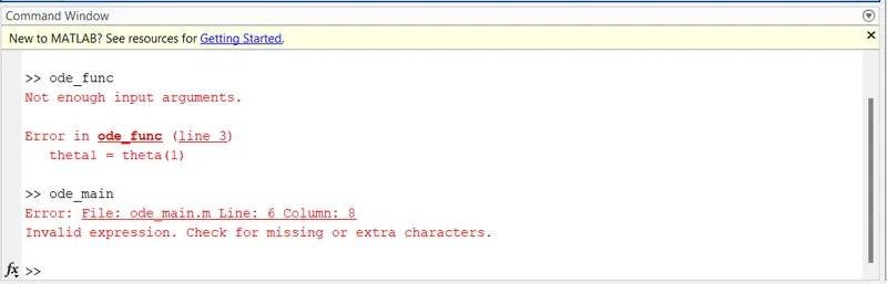
Errors:

Calling A Function Code:

function [result] = ode_func(t,theta,b,g,l,m)

   theta1 = theta(1);
   theta2 = theta(2);
   dtheta1_dt = theta2;
   dtheta2_dt = -(b/m)*2-(g/l)*sind(theta1);
   result = [dtheta1_dt; dtheta2_dt];
end   

Results:

The motion between 0-20 Sec As per given data,As Shown in figure below.

Animation:

https://youtu.be/qNeGYCUXCZU

or

https://youtu.be/qNeGYCUXCZU

Coclusion:

So it can be appli cable on Many Sectors like,

Population Growth and Decay.

Newton's Law of Cooling.

Glucose Absorption by the Body.

Spread of Epidemics.

Newton's Second Law of Motion.

Interacting Species: Competition.