Project 2 - Rankine cycle Simulator

Aim :

To Create a Rankine Cycle Simulator using OCTAVE/MATLAB.

Tasks :

1. Your code should calculate the state points of the Rankine Cycle (any type of your choice) based on user inputs.
2. Then, plot the corresponding T-s and h-s plots for the given set of inputs. Title and axes labels are a must, while legends could be used if necessary.
3. Explaining the working of a rankine cycle simulator.
4. Step-wise explanation of code.
5. Mention the errors faced while programming.
6. Screenshots showing errors thrown in command window.
7. Net work output
8. Back work ratio

Rankine cycle :

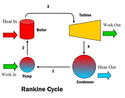
It is an idealized thermodynamic cycle describing the process by which certain heat engines, such as steam turbines or reciprocating steam engines, allow mechanical work to be extracted from a fluid as it moves between a heat source and heat sink.The line Diagram of Rankine Cycle As Shown in Fig.below.

Processes in the Rankine cycle :

The states are identified by numbers (in brown) in the T–s diagram.

Process 1–2 :

The working fluid is pumped from low to high pressure. As the fluid is a liquid at this stage, the pump requires little input energy. Process 1-2 is isentropic compression.

Process 2–3 :

The high-pressure liquid enters a boiler, where it is heated at constant pressure by an external heat source to become a dry saturated vapour. The input energy required can be easily calculated graphically, using an enthalpy–entropy chart (h–s chart, or Mollier diagram), or numerically, using steam tables or software. Process 2-3 is constant pressure heat addition in boiler.

Process 3–4 :

The dry saturated vapour expands through a turbine, generating power. This decreases the temperature and pressure of the vapour, and some condensation may occur. The output in this process can be easily calculated using the chart or tables noted above. Process 3-4 is isentropic expansion.

Process 4–1 :

The wet vapour then enters a condenser, where it is condensed at a constant pressure to become a saturated liquid. Process 4-1 is constant pressure heat rejection in condenser.

Variables :

	Heat flow rate to or from the system (energy per unit time)
	Mass flow rate (mass per unit time)
	Mechanical power consumed by or provided to the system (energy per unit time)
	Thermodynamic efficiency of the process (net power output per heat input, dimensionless)
	Isentropic efficiency of the compression (feed pump) and expansion (turbine) processes, dimensionless
	The "specific enthalpies" at indicated points on the T–s diagram
	The final "specific enthalpy" of the fluid if the turbine were isentropic
	The pressures before and after the compression process

Formulas To Remember :

In general, the efficiency of a simple rankine cycle can be written as

Each of the next four equations^[1] is derived from the energy and mass balance for a control volume. defines the thermodynamic efficiency of the cycle as the ratio of net power output to heat input. As the work required by the pump is often around 1% of the turbine work output, it can be simplified.

Required Inputs:

Turbine Inlet temperature = 400° C

Turbine Inlet Pressure = 30 bars

Turbine Outlet Pressure = 0.05 bars = Condenser Inlet Pressure

Main Code:

clear all
close all
clc
% Necessary Inputs
p1 = input('Enter the Pressure at the Turbine inlet(in bar):');
T1 = input('Enter The Temparature at turbine inlet:');
p2 = input('Pressure at Condenser inlet:');

% Finding of Cp at p1
high_cpl = XSteam('cpL_p',p1);

% state variable at point 1
disp(' variable at point 1:')
fprintf('p1  :%f barn',p1)
T1s = XSteam('Tsat_p' ,p1);
s1s = XSteam('sV_p',p1);
s1f = XSteam('sL_p',p1);
h1 = XSteam('h_pT',p1,T1);
fprintf('h1  :%f kJ/kg n' ,h1)
s1 = XSteam('s_pT',p1,T1);
fprintf('s1  : %f KJ/kgk n',s1)
fprintf('T1  : %f Deg celsius n',T1)


%state variable at point 2
disp('variable at state pint 2:')
fprintf('p2  :%f bar n',p2)
s2 = s1;
hg2 = XSteam('hV_p',p2);
hf2 = XSteam('hL_p',p2);
sg2 = XSteam('sV_p',p2);
sf2 = XSteam('sL_p',p2);
x2 = (s2-sf2)/(sg2-sf2);
h2 = hf2+x2*(hg2-hf2);
fprintf('h2  : %f KJ/kg n',h2)
fprintf('s2  : %f KJ/KgK n',s2)
T2 = XSteam('Tsat_p',p2);
fprintf('T2  : %f Deg celsius n',T2)

% State Variable at point 3
disp('variable at state pint 3:')
p3 = p2;
fprintf('p3 :%f bar n',p3)
hf3 = XSteam('hL_p',p3);
h3 = hf3;
fprintf('h3 :%f KJ/kgk',h3)
sf3 = XSteam('sL_p',p3);
s3 = sf3;
fprintf('s3 :%f KJ/kgk',s3)
T3 = T2;
fprintf('T3 : %f Deg celsius n',T3)

% State Variable at point 4
disp('variable at state pint 4:')
p4 = p1;
fprintf('p4 :%f bar n',p4)
s4 = s3;
hf4 = XSteam('h_ps',p4,s4);
h4 = hf4;
fprintf('h4 :%f KJ/kgk n',h4)
fprintf('s4 :%f KJ/kgk n',s4)
T4 = T1s/exp((s1f-s4)/high_cpl);
fprintf('T4 : %f Deg celsius n',T4)

T5 = T1s;
s5 = XSteam('sL_T',T5);

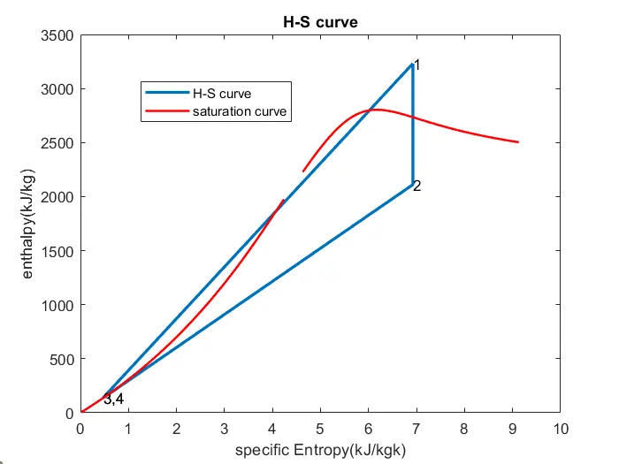
% Plotting H-S curve
figure(1)
plot([s1 s2 s3 s4 s1],[h1 h2 h3 h4 h1],'LineWidth',2)
xlabel('specific Entropy(kJ/kgk)')
ylabel('enthalpy(kJ/kg)')
title('H-S curve')
text(s1,h1,'1')
text(s2,h2,'2')
text([s3 s4],[h3 h4],'3,4')
hold on

% Invent Saturation Line
Tc = linspace(1,373,500)
for i = 1:length(Tc)
    % sat Liq Line
    hl(i) = XSteam('hL_T',Tc(i));
     sl(i) = XSteam('sL_T',Tc(i));
     % sat vap Line
    hv(i) = XSteam('hv_T',Tc(i));
     sv(i) = XSteam('sv_T',Tc(i));

end

% Plotting Saturation line
plot(sl,hl,'r','linewidth',1.5)
plot(sv,hv,'r','linewidth',1.5)
legend('H-S curve','saturation curve')

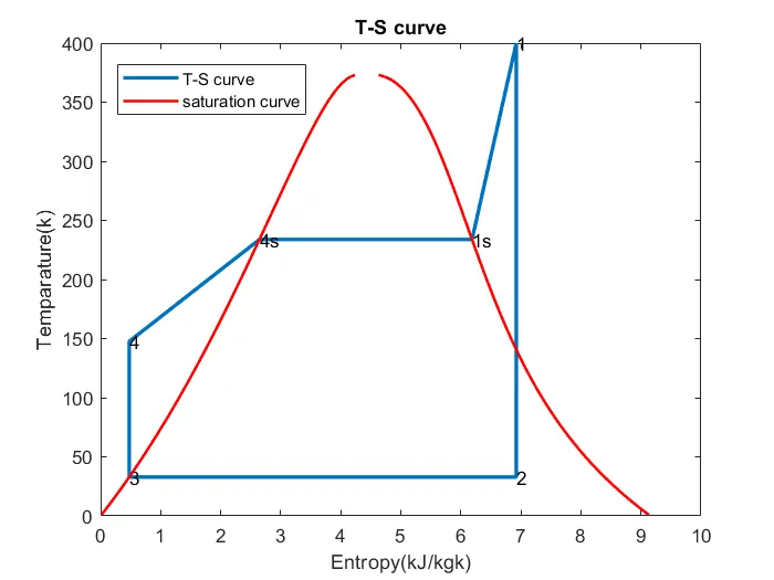
figure(2)
plot([s1 s2 s3 s4 s1f s1s s1],[T1 T2 T3 T4 T5 T1s T1],'LineWidth',2)
xlabel('Entropy(kJ/kgk)')
ylabel('Temparature(k)')
title('T-S curve')
text(s1,T1,'1')
text(s2,T2,'2')
text(s3,T3,'3')
text(s4,T4,'4')
text(s1s,T1s,'1s')
text(s1f,T5,'4s')
hold on

% Plotting Saturation line
plot(sl,Tc,'r','linewidth',1.5)
plot(sv,Tc,'r','linewidth',1.5)
legend('T-S curve','saturation curve')

% Work dobne by the turbine
Wt = h1 - h2

% Work dobne by the Pump
Wp = h4 - h3

% Net Work Done
Wnet = Wt-Wp;
fprintf('net work : %f kJ/kg n', Wnet)

% Back work Ratio
B.W.R = -Wp/Wt;
fprintf(' back work ratio : %n',B.W.R)

% Heat Addition
Qin = h1 -h4;

%thermal efficiency
TE = Wnet*100/Qin;
fprintf('thermal efficiency : %f percent ',TE)

Errors :

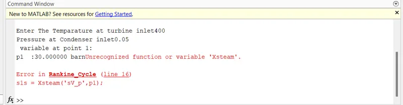
Calling Wrong Function 'Xsteam' Leads to error.

i.e.., the right function is 'XSteam' .

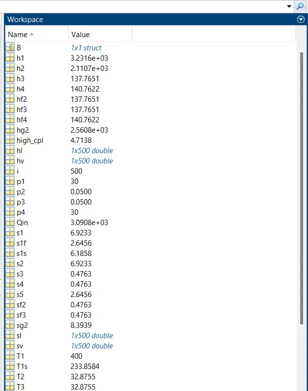
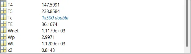
Reduced Errors Leads To Stable Outputs :

Explanation Of Coding Logic :

1. Taking the Required Inputs.
2. First, consider the pump.
3. Then Calculate The work required by the pump.
4. After the work required by the pump is calculated.
5. The enthalpy value after the pump (point 2) can be calculated.
6. Then Calculate The enthalpy at point two.
7. Similarly Specific Heat & Entropy with respective points.
8. Next, lets consider the boiler.
9. The heat input by the boiler is calculated.
10. Now, we consider the turbine.
11. The quality of the low pressure steam & the work generated by the turbine Calculated.
12. The heat rejected by the condenser is calculated.
13. We can now calculate the thermal efficiency As Well As Net Workdone.
14. Plot the figures With Proper Labelling & titles.

Plotting The Results :

H-S Curve Of Rankine Cycle:

T-S Curve Of Rankine Cycle:

Conclusion:

Rankine cycle Effectively Utilises The heat engines, ideal cyclical sequence of changes of pressure and temperature of a fluid, such as water, used in an engine, such as a steam engine. It is used as a thermodynamic standard for rating the performance of steam power plants.