Week 3 - Solving second order ODEs

AIM: To write a Matlab program to simulate the motion of a simple pendulum with damping

Simple Pendulum:
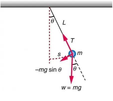
A simple pendulum has a small-diameter bob and a string that has a very small mass but is strong enough not to stretch appreciably. The linear displacement from the pendulum is s, the length of the arc. Also shown are the forces on the bob, which result in a net force of -mg sinθ toward the equilibrium position that is, a restoring force.

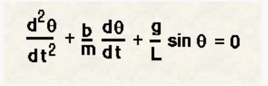
In the above equation,
g = gravity in m/s2,
L = length of the pendulum in m,
m = mass of the ball in kg,
b=damping coefficient.

Input Values:

• L=1 metre,
• m=0.1 kg,
• b=0.05.
• g=9.81 m/s2.

Convert 2nd degree ODE order into first degree ODE
Ɵ = Ɵ1
dƟ/dt = dƟ1/dt = Ɵ2
dƟ/dt+b*Ɵ/m+g*sinƟ1/L

Code for function:-

function [dtheta_dt] = ode_fun(t,theta,b,g,l,m)
         
theta1 = theta(1)
theta2 = theta(2)
dtheta1_dt = theta2;
dtheta2_dt = -(b/m)* theta2 -(g/l)*sin(theta1);
dtheta_dt = [dtheta1_dt; dtheta2_dt];


end

Code for simple pendulum program:

clear all
close all
clc



b = 0.05;
g = 9.81;
l = 1;
m = 1;


%INITIAL CONDITION
theta_0 = [0;3];


%time points
t_span = linspace(0,20,400);

%solve ode
[t , results] = ode45(@(t,theta)ode_fun(t,theta,b,g,l,m),t_span, theta_0);
i = 1
figure(1)
grid on
plot(t,results(:,1))
hold on
plot(t,results(:,2))
xlabel('time')
ylabel('plot')
legend('change in displacement', 'change in angular velocity')

for i = l:length(t)
x = (sin(results(i,1)));
y = (-cos(results(i,1)));


figure(2)
plot([0, x],[0, y],'-o')
axis ([-1 1 -2 0])
text(0, -1.6, ['time', num2str(t(i,1))])
M(i) = getframe(gcf);
pause(0.1)

end
movie(M)
videofile = VideoWriter('s_pendulum.avi','Uncompressed AVI');
open(videofile)
writeVideo(videofile,M)
close(videofile)

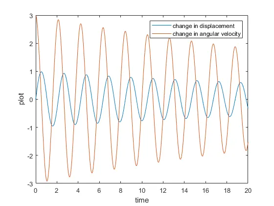
Result plot:-

Animation link:-

https://youtu.be/e7URih63xko