Week 3 - Solving second order ODEs

Solving second order ODEs: -

`(d^2 θ)/(dt^2 )+b/m (dθ)/(dt)+g/l sinθ=0` .............................

i) Converting this equation in single ODEs

1. `θ=θ1`
2. `(dθ)/(dt)=(dθ1)/(dt) = θ2` .......... 1
3. `(d^2 θ)/(dt^2 )=(d^2 θ1)/(dt^2 )=d/dt((dθ1)/(dt))= d/dt(θ2)` .......................2

equation a can be written as

`(d^2 θ1)/(dt^2 )+b/m (dθ1)/(dt)+g/l sinθ1=0`

`(dθ2)/dt+b/m (θ2)+g/l sinθ1=0` .................. 3

`(dθ1)/dt = θ2`..................... A

`(dθ2)/dt=-b/m (θ2)-g/l sinθ1` ..................... B

`d/dt [■(θ1@θ2)]=[■(θ2@-b/m θ2-g/l sinθ1)]` this is in the matrix form,

1. Writing function for the get the time and velocity at different point’s

[dtheta_dt] = ode_func(t,theta,b,g,l,m)

Where ode_func is a function name

t and theta are the variables

b = Damping coefficient

g = gravity in m/sec^2

l = length of the pendulum in m

m = mass of the pendulum in Kg

L = length of the sting

Writing the A and B and solution vector

1. Using ode45 to solve the ODE

• Ode is a solver of any differential order equation and it is 4^th R-K method
• Ode 45 one we used for solving the second order equation,
• [t,y] = ode45(odefun,tspan,y0)
• Ode 45 must have 2 inputs and 3 parameters

1) integration variables and function

2) time span 0 to 20 sec

3) initial condition (initial angular displacement and angular velocity)

• Plotting has done by plotting time and velocity to observe the damping

1. Pendulum animation

By using the for loop, we can create the animation

Counter is used to get counting the figures

• By tracking the time span, we can get all frame
• And to create the animation one end has to be fixed
• That we can obtain by initial position called x0=y0=0
• And for the length of string, we to use the trigonometry
• x1=L*sin(result(i,1));
• y1=-L*cos(result(i,1));
• above equation are create the length of string

1. plotting will use to create the simple pendulum

• creating the supportive length in the plane called X-y plane

plot ([-1 1], [0 0]

• creating the string
• by using the ‘markersize’ command we created 2 spheres
• one at fixed end ‘X0 Y0’
• another at the final end ‘X1 Y1’
• giving the ct = ct+1 it will get the frame +1 at the count
• hold on command is used to run the program smoothly

1. by using the movie command, we created animation

error faced in writing the code,

• Got error in the result as ‘NaN’ due to wrong inputs are given
• Simple mistakes by mistype,
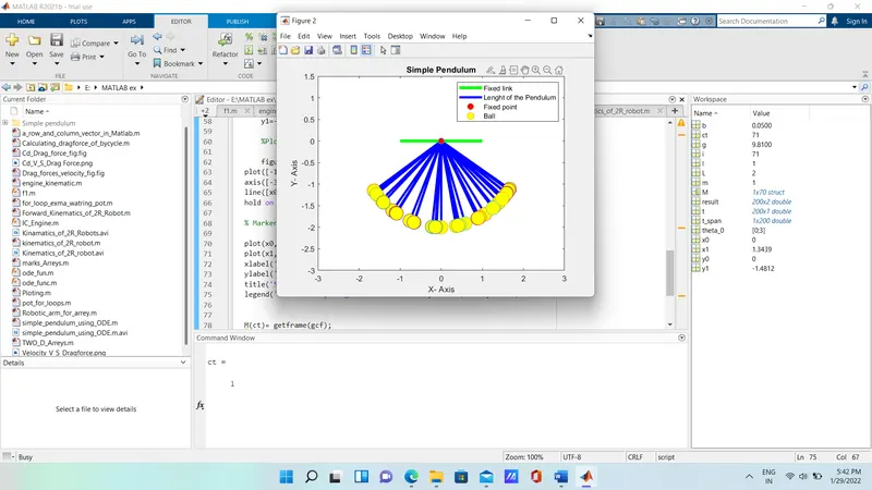
• got non – smooth animation in the figure 2
• due to hold on command is not used the old record simply printed on the graph,
• semicolon missed in the column vectors,

programing,

%% writing the program for simple pendulum 

clear all 
close all 
clc

%% geometrical parameter of  pendulum

b = 0.05;  %damping coefficient 
g = 9.81;  %gravity in m/sec^2 
l = 1;     %length of the pendulum in m 
m = 1;   % mass of the pendulum in Kg  



%% initial condition 

theta_0 = [0;3];  % initial displacement and velocity

%% Time for trace the pendulum 

t_span = linspace(0,20,200);  % calculating the pendulum for 20 sec 

%% Using solver 'ode45' to solve the ODE 
% For ode45 we need 3 parameter and 2 input 
% here (t,theta) are variables used in the function, 

[t,result] = ode45(@(t,theta) ode_func(t,theta,b,g,l,m),t_span,theta_0);

%% Plotting time and velocity 

figure (1)
plot(t,result(:,1),'LineWidth',1);
hold on 
plot(t,result(:,2),'LineWidth',1);
plot([0 20],[0 0],'LineStyle','--','Color','g')
legend('Time','Velocity','Axis')
title('Time and Velocity')
xlabel('X- Axis')
ylabel('Y- Axis')
hold off


%% Creating the animation

ct = 1 % Counter is used to getting each frame, 
L = 2; % length of the string

% Loop used to get multiple frame
for i = 1:length(t_span) % i is the variable 

    % initial variables of the string at fixed point 
    x0 = 0;
    y0 = 0;

    % Final variables of the string 
    x1=L*sin(result(i,1)); 
    y1=-L*cos(result(i,1));

    %Plotting to looks like pendulum 

    figure (2)
plot([-1 1],[0 0],'linewidth',4,'Color','g'); % plotting  fixed point
axis([-3 3 -3 1.5]);
line([x0 x1],[y0 y1],'linewidth', 3, 'color','b');% plotting string 
hold on

% Marker size command used to create the sphere 

plot(x0,y0,'O','markersize',8, 'markerfacecolor','r'); % plotting the hinged point 
plot(x1,y1,'O','markersize',18,'MarkerFaceColor','y'); % plotting the mass 
xlabel('X- Axis')
ylabel('Y- Axis')
title('Simple Pendulum')
legend('Fixed link','Lenght of the Pendulum','Fixed point','Ball')
hold off

M(ct)= getframe(gcf);
ct = ct+1;

end 
% Creating the AVI using the Movie command 
movie(M)
videofile = VideoWriter('simple_pendulum_using_ODE.m','Uncompressed AVI');
open(videofile)
writeVideo(videofile,M)
close(videofile)

youtube inks of animation

https://youtu.be/wy3xwL87ldw

results,

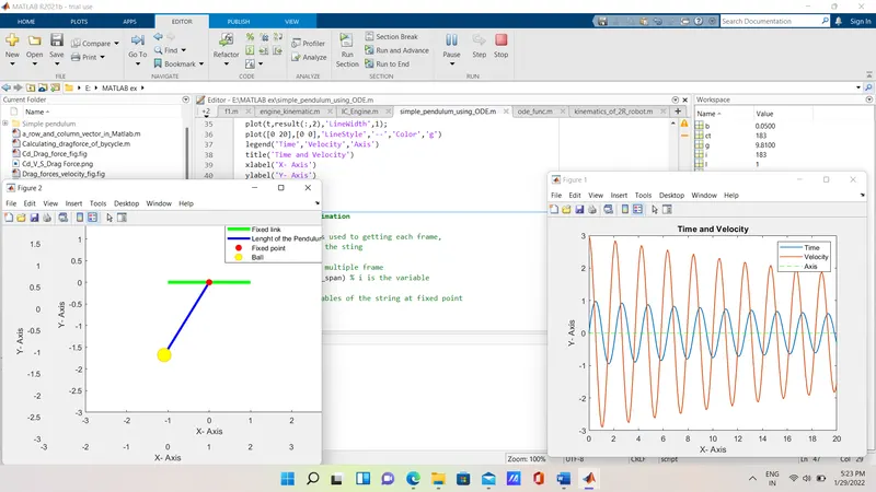
error,