Project 2 - Rankine cycle Simulator

RANKINE CYCLE SIMULATOR using MATLAB

Aim:

To create a program that simulates the state point of Rankine cycle form the input and calculates the performance parameters such as thermal efficiency, Back ration turbine and pump work.

Objective:

1. To collect the inlet turbine pressure, outlet turbine pressure and boiler temperature.
2. Using the data calculate the state points and calculate enthalpy and entropy of system.
3. Calculate the performance
4. Draw T-S diagram and H-S diagram from the calculated data.

Introduction to Rankine cycle:

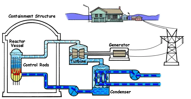
The Rankine cycle is also known as Rankine vapor cycle, this cycle is used widely for coal fired plants or nuclear powerplant. The Rankine cycle is an idealized thermodynamic cycle describing the process by which certain heat engines, such as steam turbines or reciprocating steam engines, allow mechanical work to be extracted from a fluid as it moves between a heat source and heat sink.

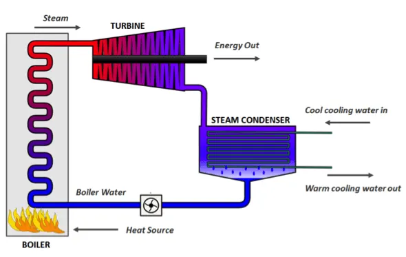
The steps in the Rankine Cycle,

process 1-2: Isentropic Expansion @Turbine

process 2-3: Isobaric Heat Rejection @Condensor

process 3-4: Isentropic Expansion @Pump

process 4-1: Isobaric Heat addition @Boiler

Components:

• Pump => Compression of fluid to high pressure.
• Boiler => High pressure liquid to vapor at high temperature and pressure.
• Turbine => Expansion of high pressure and high temperature steam to generate work.
• Condenser=> Condensation or cooling of expanded vapor.

Since water is used as working fluid the efficiency of Rankine cycle due to the efficiency of Rankine cycle is limited due to the high heat of vaporization of water. The working fluid is to be recycled and reused constantly.

Formula used

Pump= Wp = h4 – h3

Boiler = Qin = h1 – h4

Turbine= Wt = h1 – h2

Condenser = Qout = h2 - h3

Wnet = Qin – Qout

Animation of Rankine Cycle,

code

%% writing the simulator for Rankine - Cycle

clear all 
close all 
clc 

%%Cycle process

disp('          Rankine Cycle             ')
disp('Rankine cycle consist of 4 process as below')
disp('process 1-2 : Isentropic Expansion in @Turbine')
disp('process 2-3 : Isobaric Heat Rejection @Condensor')
disp('process 3-4 : Isentropic Expansion @Pump')
disp('process 4-1 : Isobaric Heat addition @Boiler')

%% obtaining the input data

p1 = input('Value of pressure at turbine inlet, p1(in bar)= ');
t1 = input('Value of Temperature at turbine inlet ,t1(in degree C)= ');
p2 = input('Value of Pressure at condenser inlet, p2(in bar)= ');

p4 = p1;

p3 = p2;

% defining data variable at state 1 

s1 = XSteam('s_pT',p1,t1);
s2 = s1;
sf2 = XSteam('sL_p',p2);
sg2 = XSteam('sV_p',p2);
sfg2 = sg2 - sf2;
x2 = (s1 - sf2)/sfg2;

if (x2 > 1)
    t2 = XSteam('T_ps',p2,s2);
    t_2 = XSteam( 'Tsat_p',p2);
    t3 = t_2;
    Td = linspace(t2,t_2,50);
    s_2 = XSteam('sV_T',t_2);
    s3 = XSteam('sL_T',t3);
    s4 = s3;
else 
    t2 = XSteam('Tsat_p',p2);
    t_2 = t2;
    t3 = t2 ;
    s3 = sf2;
    s4 = s3;
end
 
% Calculating the enthalpy 
h1 = XSteam('h_pT',p1,t1);
hf2 = XSteam('hL_p',p2);
hg2 = XSteam('hV_p',p2);
hfg2 = hg2 - hf2 ;
h2 = hf2 + x2*hfg2;

h3 = hf2;

v3 = XSteam('vL_p',p3);

h4 = v3*(p1-p2)*100 +h3;
cp = XSteam('cp_ps',p3,s3);
cv = XSteam('cv_ps',p3,s3);
k = 1 - (cv/cp);
t4 = t3*((p4/p3)^k);

t5 = XSteam('Tsat_p',p1);
t6 = t5 ;

s5 = XSteam('sL_T',t5);
s6 = XSteam('sV_T',t6);

% turbine work 
wd_tb = h1 -h2;

wd_pm = h4 - h3;

% net work 
W_net = wd_tb - wd_pm;

bwr = (h1 - h4)/(h2 - h3);
efficiency = W_net/ (h1 -h4);
eff= efficiency*100;



% plotting graph 
T = linspace(t6,t1,500);
for i = 1:length(T)
    S(i) = XSteam('s_pT',p1,T(i));
    H(i) = XSteam('h_pT',p1,T(i));
end
% data saturation temp curve 
maxt = linspace(1,t1,500);
for j = 1: length(maxt)
    satlS(j) = XSteam('sL_T',maxt(j));
    satvS(j) = XSteam('sV_T',maxt(j));
    satlH(j) = XSteam('hL_T',maxt(j));
    satvH(j) = XSteam('hV_T',maxt(j));
end

% T- S dai 
subplot(1,2,1)

%  plot sat curve 
plot (satlS,maxt,'Color','r')
hold on
plot (satvS,maxt,'Color','r')
plot(4.4230,373.6,'o','MarkerFaceColor','r','MarkerSize',7)

% plot  - pont t5 &t6 
plot([s5 s6],[t5 t6],'Color','k','LineWidth',2);
plot (S,T,'Color','k','LineWidth',2);
plot ([s1 s2],[t1 t2],'Color','k','LineWidth',2);

if (x2 > 1);
    for z = 1:length(Td)
        Sd(i) = XSteam('s_pT',p2,Td(i));
        Hd(i) = XSteam('h_pT',p2,Td(i));
    end

% plot of t2 and T_2 

plot(Sd,Td,'Color','k','LineWidth',2)
plot([s_2 s3], [t_2 t3],'Color','k','LineWidth',2)
else 
    plot([s2 s3],[t2 t3],'Color','k','LineWidth',2)
end

plot ([s3 s4],[t3 t4],'Color','k','LineWidth',2);

% plot constant pressure 
plot([s4 s5],[t4 t5],'Color','k','LineWidth',2);

title('T-S Diagram of Rankine Cycle')
xlabel('Entropy (KJ/K)')
ylabel('Temperature (deg C)')

text(s1,t1,"1");
text(s2,t2,"2");
if (x2 >1);
    text(s_2,t_2,"2'");
 end
text(s3,t3,"3");
text(s4,t4,"4");

% H&S dai
subplot(1,2,2)
% plot saturation curve 
plot(satlS,satlH,'Color','r','LineWidth',2)
hold on 
plot(satvS,satvH,'Color','r','LineWidth',2)

plot([s1 s2],[h1 h2],'Color','k','LineWidth',2)

if (x2 > 1)
    h_2 = XSteam('h_ps',p2,s_2);
    %ploting const pressure Q in
    plot(Sd,Hd,'Color','k','LineWidth',2)

   % const preess Q out 
    entrpy = linspace(s_2,s3,100);
    for k = 1:length(entrpy)
        enthlpy(k) = XSteam('h_ps',p2,entrpy(k));
    end
    % plot - constat Q rejcion curve
    plot (entrpy,enthlpy,'Color','k','LineWidth',2)
else 
    entrpy = linspace(s2,s3,100);
    for k = 1:length(entrpy);
        enthlpy(k) = XSteam('h_ps',p2,entrpy(k));
    end
   plot(entrpy,enthlpy,'Color','k','LineWidth',2)
end
 plot ([s3 s4],[h3 h4],'Color','k','LineWidth',2)
 entrpy1 = linspace(s4,s1,100);
 for l = 1:length(entrpy1)
     enthlpy1(l) = XSteam('h_ps',p1,entrpy1(l));

 end

plot(entrpy1,enthlpy1,'Color','k','LineWidth',2);

title('H - S Diagram of Rankine Cycle')
xlabel('Entropy(KJ/KG k)')
ylabel('Enthalpy (KJ/Kg)')

text(s1,h1,"1")
text(s2,h2,"2")
if (x2 > 1)
    text(s_2,h_2,"2'")
end
text(s3,h3,"3");
text(s4,h4,"4");


disp('At state point 1')
fprintf('P1 is : %f bar\n',p1)
fprintf('T1 is: %f Deg Celcius\n',t1)
fprintf('h1 is: %f KJ/Kg\n',h1 )
fprintf('s1 is: %f KJ/KgK\n',s1 )

disp('At state point 2')
fprintf('P2 is : %f bar\n',p2)
fprintf('T2 is: %f Deg Celcius\n',t2)
fprintf('h2 is: %f KJ/Kg\n',h2 )
fprintf('s2 is: %f KJ/KgK\n',s2)

disp('At state point 3')
fprintf('P3 is : %f bar\n',p3)
fprintf('T3 is: %f Deg Celcius\n',t3)
fprintf('h3 is: %f KJ/Kg\n',h3 )
fprintf('s3 is: %f KJ/KgK\n',s3 )

disp('At state point 4')
fprintf('P4 is : %f bar\n',p4)
fprintf('T4 is: %f Deg Celcius\n',t4)
fprintf('h4 is: %f KJ/Kg\n',h4 )
fprintf('s4 is: %f KJ/KgK\n',s4 )

disp('Calculation')
fprintf('Wt is: %f KJ/Kg\n',wd_tb)
fprintf('Wp is: %f KJ/Kg\n',wd_pm)
fprintf('Wnet is: %f KJ/Kg\n',W_net)
fprintf('Efficiency is: %f Percentage\n',eff)
fprintf('Back Work Ratio: %f',bwr)

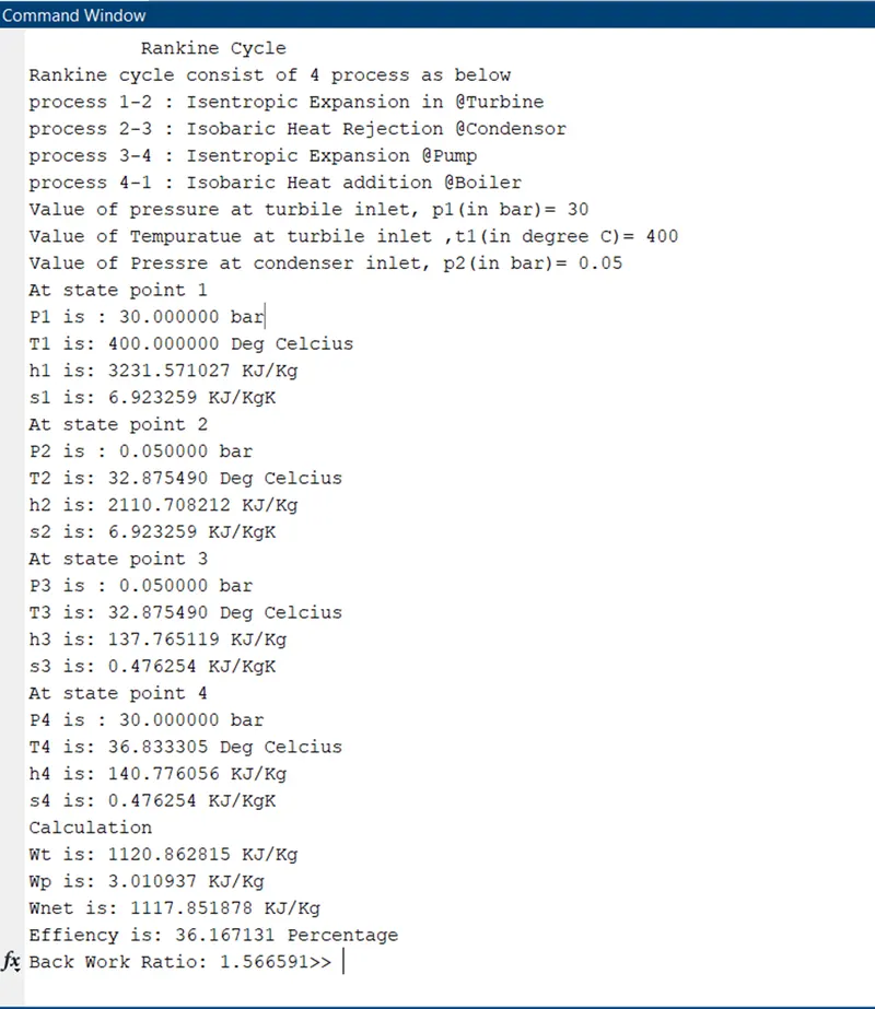
Command window,

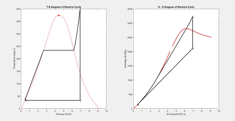
T- S & H - S Diagram,

code explanation

1. Xsteam date is used to extract steam and liquid properties of enthalpy, entropy and specific pressure and temperature,
2. For input values requires pressure at inlet of turbine and outlet of turbine and temperature at inlet,
3. By using the above data, all point variable calculated,
4. By using appropriate formulas and the data generated and performance,
5. Plotting of T-S and H-S diagram as plotted,
6. Printing of the result done by using fprintf

conclusion:

A code to simulate the rankine cycle is done with claculation for performance parameters along with plots,

Reference,

1. http://www.nuclear-power.net/nuclear-engineering/thermodynamics/thermodynamic-cycles/rankine-cycle-steam-turbine-cycle/theory-of-rankine-cycle-equations-and-calculation/#:~:text=An%20isobaric%20process%20is%20a,changes%20the%20system's%20internal%20energy.&text=In%20this%20equation%2C%20dW%20is,known%20as%20the%20boundary%20work.
2. https://en.wikipedia.org/wiki/Rankine_cycle
3. https://www.theengineerspost.com/rankine-cycle/
4. https://skill-lync.com/student-projects/Project-2-Rankine-Cycle-Simulator-95692