Solving ODE

Aim

• To write a program that solves a second degree differential equation. This second degree differential equation represents the equation of motion of a simple pendulum with damping.
• Also generate an animation describing the simple pendulum motion solved from the ODE.

Theory

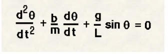
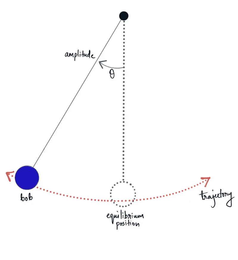
Simple pendulum works based on the principle of simple harmonic motion. Simple harmonic motion is based on Newton's second Law of motion. Which can be described by the equation given below. This equation gives the position of the bob with respect to time.

Code Procedure

Step 1

Started the code with clear all ,close all ,clc commands then defined the input parameters like mass of the bob ,length of the string , damping coefficient and acceleration due to gravity.

Step 2

Defined the initial conditions like angular velocity and displacement in the variable theta_0 as an array. Also the time period is defined in a variable called time_span with the linspace command. 0 to 20 values with 500 elements in between them and assigned it to time_span.

Step 3

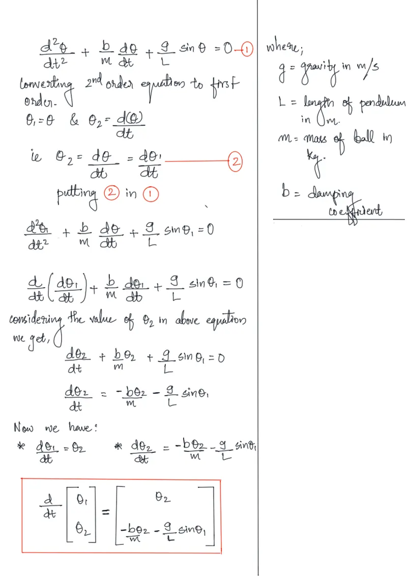
The broken down ODE is solved using the inbuilt function called ODE45.

[t, results] = ode45(@(t,theta) ode_func(t, theta, b,g,l,m),t_span, theta_0);

Here,

0de45 is the function name

T and theta are the dependent variables of the function. Alternatively we can say that ode is the function of t,theta

Now a custom function called ode_func* is defined to pass on the input parameters to the ode45 function.

Then we provide the initial parameters and the integration

*ode_func custom MATLAB function

In this function the broken down ode is defined in different variables and the values are stored according to the input parameters.

Step 4

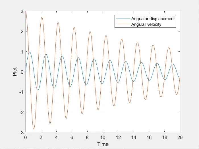
The graph which shows the angular displacement and velocity with respect to time is plotted.

Step 5

Using for loop, the pendulum motion animation is created. In the for loop the range is set from 1 to the length of the result variable which contains the angular displacement values. Then for the upper base axis , x0 and y0 are defined . x1 and y1 are defined for the string.

Step 6

The resulting animation is saved as an AVI file by getting the frame with getframe command then it is converted into video with videoWriter command along with openvideo and closevideo commands.

MATLAB Code

% A program to solve the 2nd order ODE

clear all
close all
clc

b = 0.05;
g = 9.81;
l = 1;
m = 0.5;

% Initial condition
t_span = linspace (0,20,500);

% Time points
theta_0 =[0;3];

% Solving the ODE
[t, results] = ode45(@(t,theta) ode_func(t, theta, b,g,l,m),t_span, theta_0);

figure(1)
plot(t,results(:,1))
hold on
plot (t,results(:,2))
ylabel('Plot')
xlabel('Time')
legend('Angualar displacement','Angular velocity');

ct =1;
for i = 1:length(results(:,1))
    x0 = 0;
    y0 = 0;
    
    %Definition of ball in x direction
    x1 = l*sin(results(i,1));
    
    %Definnition of ball in y direction
    y1 = -1*cos(results(i,1));
    
    
    %Plotting the Simple pendulum motion animation
    
    figure(2)
    
    %upper Base line definintion 
    plot([-0.5,0.5],[0,0],'linewidth',3,'color','g');
    hold on
    
    %Pendulum string definition 
    plot([x0 x1],[y0 y1],'linewidth',1,'color','b');
    
    %Pendulum ball definition 
    plot(x1,y1,'marker','o','markerface','r','markersize',15);
    
    %fixing the axis
    axis([-2,2,-2,2]);
    
    title('Simple Pendulum Oscillation');
    pause(0.0);
    hold off
    
    %Getting the frames generated from the loop by the ct variable
    M(ct)= getframe(gcf);

    %Iterating ct variable in the for loop
    ct = ct+1;
end

 movie(M) 
 
%Defining the videoout's filename and format using videoWriter funtion 
 videofile = VideoWriter('Simple_pendulum.avi','uncompressed AVI');
 
 %opening the video file
 open(videofile)
 
 %writing the captured frames in M into the video file
 writeVideo(videofile,M)
 
 %Closing the video file
 close(videofile)
        

ode_func custom MATLAB code

function [dtheta_dt] = ode_func(t,theta,b,g,l,m)

    theta1 = theta(1)
    theta2 = theta(2)
    dtheta1_dt = theta2;
    dtheta2_dt = -(b/m)*theta2 - (g/1)*sin(theta1);
    dtheta_dt = [dtheta1_dt; dtheta2_dt];
end

Output

Result

• A program that solves a second degree differential equation is successfully executed.
• Also generated an animation describing the simple pendulum motion solved from the ODE.