Week 3 - Solving second order ODEs

AIM :

• To write a program in MATLAB tha solves ODE which represents the equation of motion of a simple pendulum with damping.
• To write a MATLAB program that will stimulate the pendulum motions.

Theory :

In mathematics, the term Ordinary Differential Equations also known as ODE is an equation that contains only one independent variable and one or more of its derivatives with respect to the variable. In other words, the ODE is represented by as the relation having one independent variable x, the real independent variable y, with some of its derivatives.

The order of ordinary differential equations is defined to be the order of the highest derivative that occurs in the equation. The general form of n-th order ODE is given as;

F(x, y,y’,….,y^n ) = 0

Note that, y’ can be either dy/dx or dy/dt and y^n can be either d^ny/dx^n or d^ny/dt^n.

An n-th order ordinary differential equations is linear if it can be written in the form;

a₀(x)y^n + a₁(x)y^n-1 +…..+ a_n(x)y = r(x)

The function a_j(x), 0 ≤ j ≤ n are called the coefficients of the linear equation. The equation is said to be homogeneous if r(x) = 0. If r(x)≠0, it is said to be a non- homogeneous equation.

The ordinary differential equation is further classified into three types. They are:

• Autonomous ODE
• Linear ODE
• Non-linear ODE

The way pendulum moves depends on the Newtons second law. When this law is written down, we get a second order differential equation that describes the position of the ball w.r.t time.

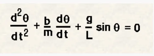
In the above equation,

g = gravity in m/s^2

L = Length of the pendulum in m

m = mass of the ball in kg

b = damping coefficient

A damping coefficient is a material property that indicates whether a material will bounce back or return energy to a system. For example, a basketball has a low damping coefficient. If the bounce back is cause by unwanted vibration or shock, a high damping coefficient in the material will diminish the response. It will swallow the energy and reduce the undesired reaction.

SOLVING 2ND ORDER ODE USING MATLAB :

ODE of damped pendulum is 2nd order ordinary differential equations, so we have to convert it into first order ODE.

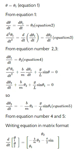
Now, after the conversion we have to use MATLAB solver ode45 to solve the equation.

OBJECTIVES :

1. Solve ODE which represents equation motion of simple pendulum with damping using MATLAB code.
2. Explaining the flow and content in the program.
3. Creating an animation plot of for motion of pendulum from the given data.

PROGRAM

close all
clear all
clc

%Given data : %Length(L) = 1 metre
              %Mass of the ball(m) = 1 kg
              %Damping coefficient(b) = 0.05
              %Gravity(g) = 9.81 m/s^2
b=0.05;
g=9.81;
L=1;
m=1;

%Initial condition :
%Initial angular displacement = 0; initial angular velocity = 5 rad/sec

theta_0 = [0;5];


%Time points

t_span = linspace(0,20,500);

%Solving ODE

[t, results] = ode45(@(t,theta) ode_func(t_span, theta, b,g,L,m),t_span, theta_0);
plot(t, results(:,1));
hold on;
plot(t, results(:,2));
ylabel('Amplitude');
xlabel('Time');
legend('Angular displacement in rad','Angular displacement in rad/s');
grid on;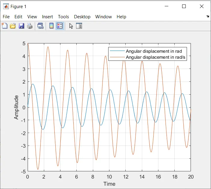

From above graph it can be observed that oscillation of pendulum are gradually damped as we can observe that angular displacement and angular velocity was gradually decreasing with time.

-------------------------------------------------------------------------------------------------------------------------------------------

Now the below code will help us in stimulating animations of damped pendulum.

PROGRAM

close all
clear all
clc

%Given data : %Length(L) = 1 metre
              %Mass of the ball(m) = 0.1 kg
              %Damping coefficient(b) = 0.05
              %Gravity(g) = 9.81 m/s^2
b=0.05;
g=9.81;
l=1;
m=0.1;

%Initial condition :
%Initial angular displacement = 0; initial angular velocity = 5 rad/sec

theta_0 = [0;5];

%Time points

t_span = linspace(0,20,500);

%Solving ODE

[t, results] = ode45(@(t,theta) ode_func(t_span, theta, b,g,l,m),t_span, theta_0);
figure(1)
plot(t, results(:,1));
hold on;
plot(t, results(:,2));
ylabel('Amplitude');
xlabel('Time');
legend('Angular displacement in rad','Angular displacement in rad/s');
grid on;
figure(2)
ct=1;

%Using For loop

for i=1:length(results(:,1))
    x0=0;
    y0=0;
    plot([-1 1],[0,0],'linewidth',4,'color','k');
    hold on

%Position of the ball

x1=l*sin((results(i,1)));
%Because (0,0) is fixed point, x1 will be on the right side during the start.
y1=-l*cos((results(i,1))); 
%Because (0,0) is fixed point, y1 will be below during the start.

%Plotting the length of the pendulum

plot([x0,x1],[y0,y1],'linewidth',2,'color','r');

%Plotting of the fixed end

plot(x0,y0,'-s','MarkerEdgeColor','g','MarkerFaceColor','b','MarkerSize',10);

%Plotting of the ball

plot(x1,y1,'-o','MarkerEdgeColor','g','MarkerFaceColor','c','MarkerSize',20);
hold off
grid on
titlestring=['Pendulum motion at time t=',num2str(t(i)),'seconds'];
title(titlestring, 'fontsize',10);
axis([-1.5 1.5 -1.5 1.5])
M(ct)=getframe(gcf);
ct=ct+1;
end

%Animation of the pendulum motion

movie(M)
videofile=VideoWriter('ordinarydifferentialequation.avi)','Uncompressed AVI');
open(videofile)
writeVideo(videofile,M)
close(videofile)

EXPLAINING THE PROGRAM :

• In the above program we can see that the code is same till adding the code to stimulate the motion of the pendulum. i.e till grid on; figure(2)
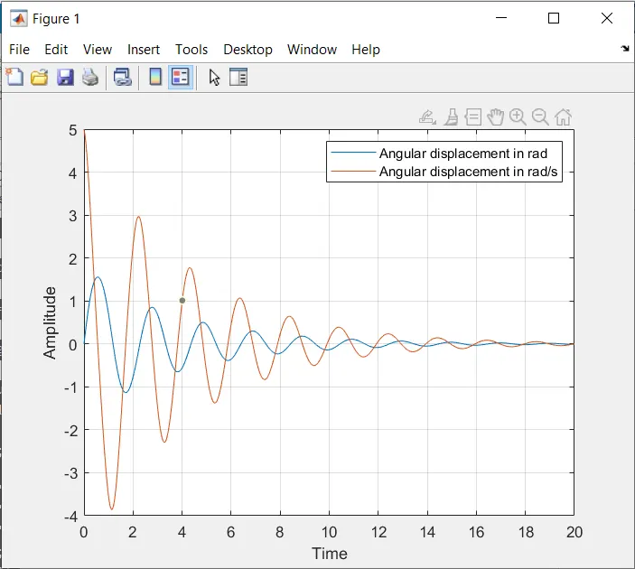
• The only change in the value of mass of the ball is changed. I have considered mass(m) = 0.1 kg here.
• Now we have 'ct' which is the counter command with a value of 1 and is getting increament by +1.
• Since, we want the motion to be continuous flow we have introduced a 'for loop' and added a variable 'i' to it.
• The loop will continue to run till the mentioned length results.
• We can also notice that there is a video file created in which we have saved the animation, for dumping out all the other data we have used 'Uncompressed AVI'. We have done this so we don't have to open MATLAB and run the program everytime we want to see the animation of the simple pendulum.
• At every next second we have a different position of the pendulum. We have assumed the length of the string and size of the pendulum. For creating the ball(sphere) we have used the marker command and mentioned various paramters like edgecolour,facecolour and size.
• I have plotted different axis co-ordinates for the simple pendulum to be placed at a proper viewable and presentable purpose.
• I have also mentioned comments before coding every content for better understanding and presentation purpose.

Below is the graphical output after plotting the results(figure 1 window)

Below are given a few screenshots of the pendulum at different time intervals.(figure 2 window)

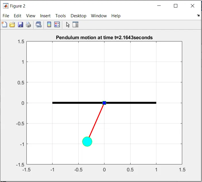
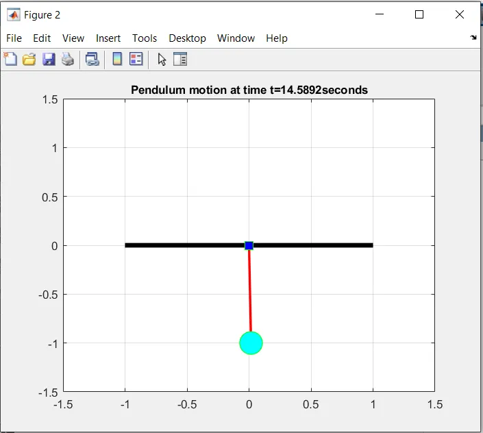
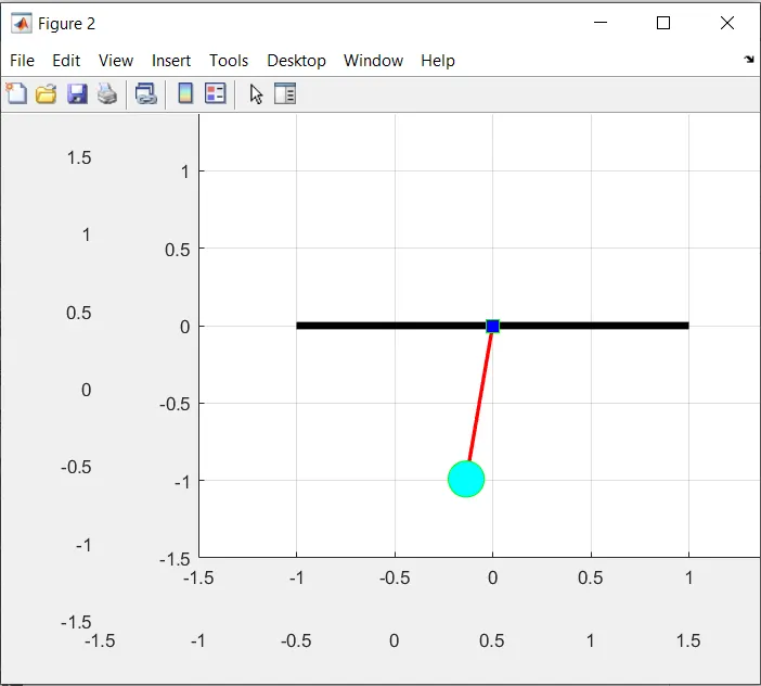
While programming this, I faced a error of which I have shared a screenshot and explained how can we resolve that error.

ERROR

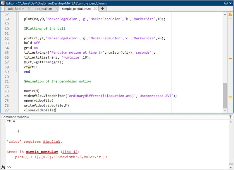
This error was thrown in the command windown because I had coded in without ' ' symbol. A 'color' specification is required if you want to add a colour of your choice. It was resolved immediately by giving proper symbols as required by simulink.

***************************************************************************************************

I have uploaded the video on Youtube and have shared the link below :

https://youtu.be/bf_GEpjg38I