AIR STANDARD CYCLE
Aim - To wirte a code that can solve an otto cycle and making plots for it.
Firstly we will get a general idea of a otto cycle with the image given below.
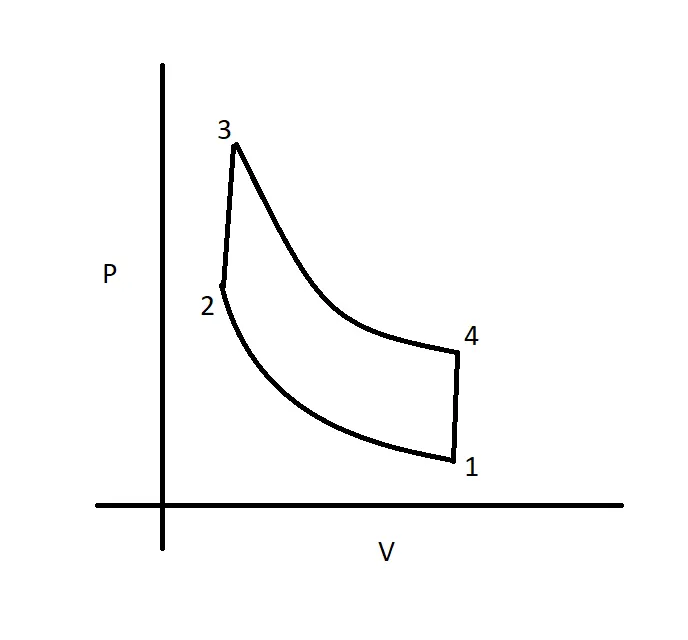
*The above image is just a rough image editted by me in paint software to explain the basics*
The above PV diagram has 4 states :
1 - 2 Isentropic compression,2 - 3 Constant volume heat addition,3 - 4 Isentropic expansion,4 - 1 Constant volume heat rejection
_______________________________________________________________________________________________________
PROGRAM
________________________________________________________________________________________
%Inputs (Temperature is in Kelvin[K], Pressure is in Pascal [Pa])
gamma=1.4
t3 = 2300

% State variables at state point 1
p1 = 101325
t1 = 500

% Engine geometric paramters
bore=0.1;
stroke=0.1;
con_rod=0.15;
cr=12;

% Calculating the clearance volume and the swept volume
v_swept = (pi/4)*bore^2*stroke;
v_clearance = v_swept/(cr-1);

v1 = v_swept + v_clearance
v2 = v_clearance

% State variable at state point 2
% p2v2^gamma = p1v1^gamma
% p2 = p1(v1/v2)^gamma = p1*cr^gamma
p2 = p1*cr^gamma;

% p1v1/t1 = p2v2/t2 | t2 = p2*v2*t1/(p1v1)
t2 = p2*v2*t1/(p1*v1);

constant_c = p1*v1^gamma
V_compression=engine_kinematics(bore,stroke,con_rod,cr,180,0)
P_compression = constant_c./V_compression.^gamma

% State variables at state point 3
v3 = v2


% p2v2/t2 = p3v3/t3 | p3 = p2*t3/t2
p3 = p2*t3/t2

constant_c = p3*v3^gamma
V_expansion = engine_kinematics(bore,stroke,con_rod,cr,0,180)
P_expansion = constant_c./V_expansion.^gamma

% State variables at state point 4
v4 = v1

% p3v3^gamma = p4v4^gamma | p4 = p3(v3/v4)^gamma
p4 = p3*(v3/v4)^gamma

figure(1)
hold on
plot(v1,p1,'*','color','r')
plot(V_compression,P_compression)
plot(v2,p2,'*','color','r')
plot(v3,p3,'*','color','r')
plot(V_expansion,P_expansion)
plot(v4,p4,'*','color','r')
plot([v2 v3],[p2 p3],'color','b')
plot([v4 v1],[p4 p1],'color','b')

figure(2)
plot([v1,v2,v3,v4],[p1,p2,p3,p4],'color','b')
EXPLANATION OF THE PROGRAM :
1. Firstly we have to consider pressure, volume and temperature at different state points are p,v,t. eg. at point 1 p1,v2 & t1 and so on for state points 2,3,4.
2. Now to calculate the clearance volume and swept volume to compute the volume at top dead centre and bottom dead centre we have to apply the basic geometric kinematics parameters bore,stroke,connecting rod length(con_rod) and the compression ratio(cr).
3. After calculting the clearance and swept volume we can compute the volumes at the top dead and bottom dead centre with generic formulae.
4. We have to assume the temperature and pressure at state point 1, with the isentropic process formula we can compute values at state point 2, and at state point 3 which is the constant volume heat combustion process we can compute the values by using ideal gas equation. At state point 3 the pressure is going to be the highest because it is a combustion process.
5. Now at state point 4, the volume of state point 1 is going to be equal to the volume at state point 4. At different state points we have used different expression and equations in order the compute the missing values of pressure or temperature.
6. After calculating all this, we will have all values at all 4 state points.So now we can plot them to obtain a PV diagram. For this first we have created a figure window and used hold on command. After plotting the points we have to join them correctly.
7. The points should be joined with correct curves but for this we will need for information on how the piston moves from top dead centre to bottom dead centre and how the values of the engine combustion chamber changes.
8. For this I have coded a seperate program in which I have used function calling method.
PROGRAM
__________________________________________________________________________________________
function [V] =  engine_kinematics(bore,stroke,con_rod,cr,start_crank,end_crank)

a = stroke/2
R = con_rod/a

v_s=pi/4*bore^2*stroke
v_c=v_s/(cr-1);

theta = linspace(start_crank,end_crank,100);

term1 = 0.5*(cr-1);
term2 = R +1 - cosd(theta);
term3 = (R^2 - sind(theta).^2).^0.5;

V = (1 + term1*(term2 - term3)).*v_c;

end
EXPLAINING THE PROGRAM.
1. In the above program first we have considered a function '[V]' which has the value of program 'engine_kinematics and the inputs of different parameter like bore,stroke,connecting rod length(con_rod) and compression ratio(cr). Now we have 2 new parameters here starting crank angle(start_crank) which is the angle made at the top dead centre and another is ending crank angle(end_crank) which is the angle made at the bottom dead centre.
2. We will compute the swept volume and clearance volume, then we will assign a variable 'theta' for the changes made in the angles. We need to compute the different angles so we use linspace command with 100 different values considered for the starting crank and ending crank(as mentioned in the program above).
3. Now we have a expression derived from geometric considerations. i.e { VVc = 1 + 12(rc - 1)[R + 1 - costheta - (R^2 - sin^2theta)^12] }
4. For simplicity of calculating we have splitted the entire expression in 3 different terms naming term1,term2 and term3.
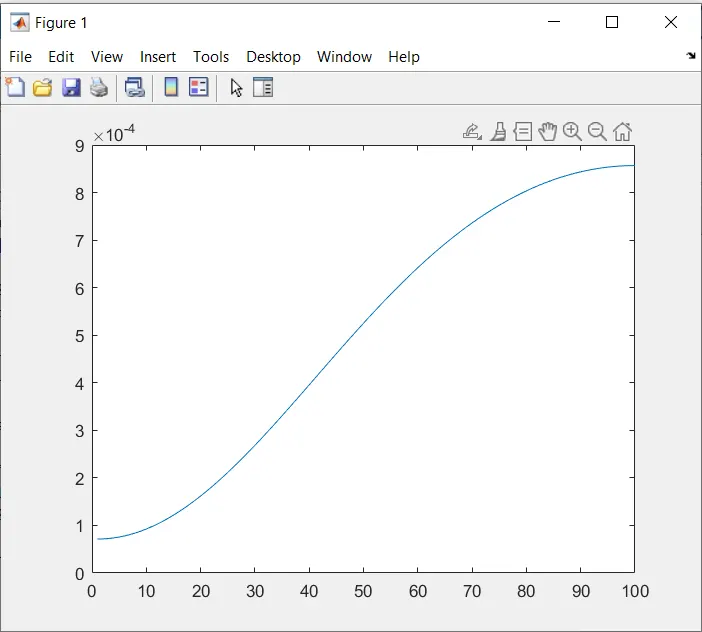
5. We can plot the array ([V]) for us to have a general idea and also if our code is running correctly.
6. Now after computing everything, we have to use the above program in our PV diagram program to calculate the Volume change during the compression and expansion stroke.
7. Referring to our PV diagram program we have used to V_compression and V_expansion at different state point variable to compute the volume changes.
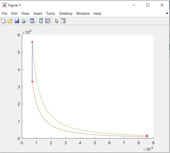
8. Now we can finally plot our PV diagram by joining all the points to get a smooth curve connecting all state points as shown in the figure below.
_______________________________________________________________________________________________________
Below are a few screenshots of outputs I got after plotting in the above programs.
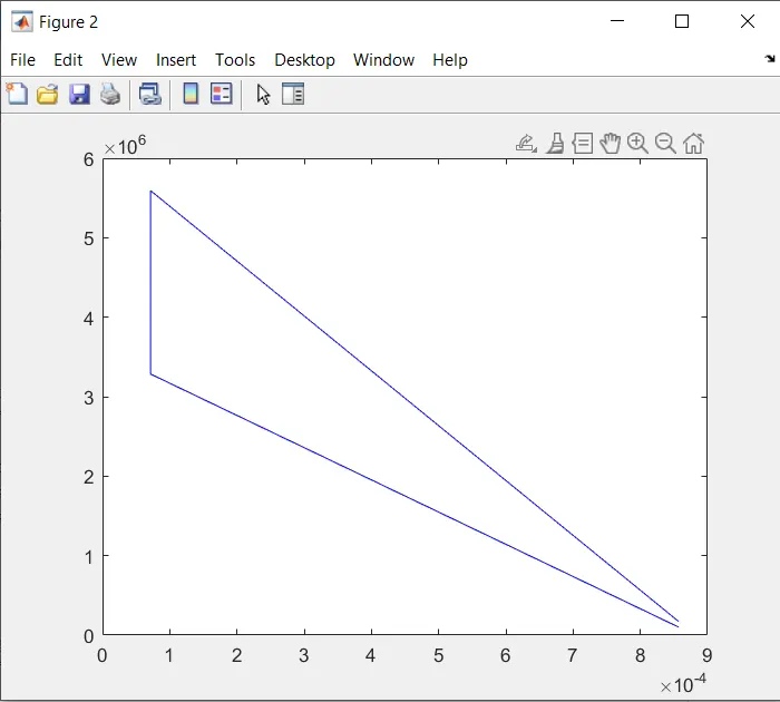
*******************************************************************************************************
OUR FINAL REQUIRED PV DIAGRAM.
_______________________________________________________________________________________________________
Now while coding these programs I faced some errors. I will share the image of the error thrown in the command window and will explain how I resolved it below the image.
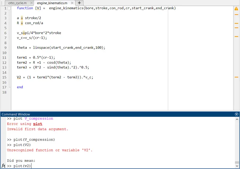
ERROR 1
I have got this error because the array function [V] (line 1) I have taken to input the values does not have the same function name [V2] (line 15).
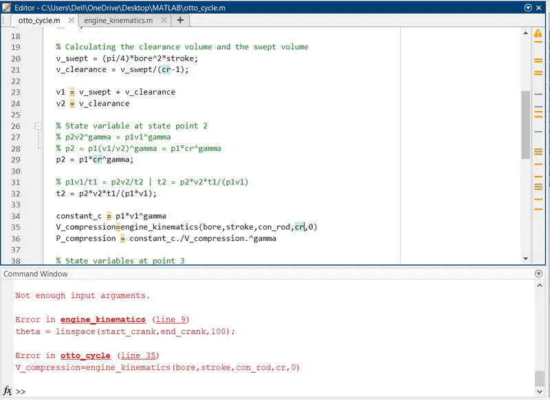
ERROR 2
I have got this error because while calculating V_compression I haven't inserted the same amount of inputs as those when I inserted during function calling.
**************************************************************************************************************************************************************************************************************
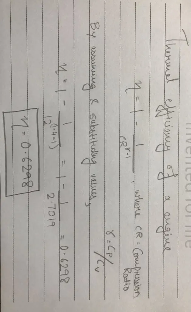
AIM - TO OUTPUT THE THERMAL EFFICIENCY OF A ENGINE
It would have not look presentable and understandable by typing the formula and substituting the values to calculate the thermal efficiency of a engine, I wrote it on a page, took a screenshot and I am uploading that image below.
------------------------------------------------------------------------------------------------------------------------------------------------