Project 2 - Rankine cycle Simulator

AIM :

To create a Rankine cycle simulator using MATLAB

OBJECTIVES :

• To create a basic program that calculates the state points
• To add the thermodynamic relation to get the points inbetween the state variables.
• To plot rankine cycle on T-s and H-s curve.

THEORY :

The Rankine cycle is an idealized thermodynamic cycle describing the process by which certain heat engines, such as steam turbines or reciprocating steam engines, allow mechanical work to be extracted from a fluid as it moves between a heat source and heat sink. The Rankine cycle is named after William John Macquorn Rankine, a Scottish polymath professor at Glasglow University.

There are four processes in the Rankine cycle.

• Process 1–2: The working fluid is pumped from low to high pressure. As the fluid is a liquid at this stage, the pump requires little input energy. Process 1-2 is isentropic compression.
• Process 2–3: The high-pressure liquid enters a boiler, where it is heated at constant pressure by an external heat source to become a dry saturated vapour. The input energy required can be easily calculated graphically, using an enthalpy-entropy chart (h-s chart, or Mollier diagram), or numerically, using steam tables or software. Process 2-3 is constant pressure heat addition in boiler.
• Process 3–4: The dry saturated vapour expands through a turbine, generating power. This decreases the temperature and pressure of the vapour, and some condensation may occur. The output in this process can be easily calculated using the chart or tables noted above. Process 3-4 is isentropic expansion.
• Process 4–1: The wet vapour then enters a condenser, where it is condensed at a constant pressure to become a saturated liquid. Process 4-1 is constant pressure heat rejection in condenser.

In an ideal Rankine cycle the pump and turbine would be isentropic, i.e., the pump and turbine would generate no entropy and hence maximize the net work output. Processes 1–2 and 3–4 would be represented by vertical lines on the T-s diagram and more closely resemble that of the Carnot cycle. The Rankine cycle shown here prevents the state of the working fluid from ending up in the superheated vapor region after the expansion in the turbine, which reduces the energy removed by the condensers.

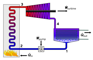
RANKINE CYCLE PROGRAM :

clear all 
close all
clc

%Displaying
disp('  RANKINE CYCLE   ');
disp('1-2 is Isentropic Expansion in the turbine');
disp('2-3 is constant pressure heat removal in the condenser');
disp('3-4  is Isentropic compression in the pump');
disp('4-1 is Constant pressure heat addition in the boiler');

%Obtaining the input data
p1=input('nValue of pressure at turbine inlet, p1(in bar)= ');
T1=input('nValue of temperature at turbine inlet, T1(in degreee)= ');
p2=input('nValue of temperature at condenser inlet, p2(in bar) = ');

%Extracting data and defining variables
%STATE 1
h1 = XSteam('h_pT', p1, T1);           %extracting enthalpy at state point 1
s1 = XSteam('s_pT', p1, T1);           %similarly

%STATE 2
s2 = s1;                               %Isentropic expansion
sf2 = XSteam('sL_p', p2);              %Saturated liquid Entropy
sg2 = XSteam('sL_p', p2);              %Saturated vapour Entropy
x2 = (s2 - sf2)/(sg2 - sf2);
hf2 = XSteam('hL_p', p2);
hg2 = XSteam('hL_p', p2);
h2=XSteam('h_ps',p2,s2);

%STATE 3
p3 = p2;                               %Constant heat rejection in the condenser
s3 = XSteam('sL_p', p3);
h3 = XSteam('hL_p', p3);

%STATE 4
s4 = s3;
p4 = p1;

%Woek done by turbine
Wt = h1 - h2;

%Work done to run pump
v3 = XSteam('vL_p', p3);
Wp = v3*(p4 - p3)*100;
h4 = h3 + Wp;

%net work
Wnet = Wt - Wp;

%Heat into the system
Qin = h1 - h4;

%Heat out of the system
Qout = h2 - h3;

%Thermal efficiency
eff = (Wnet/Qin)*100;

%Specific Steam Consumption
%SSC = mass flow rate/power
SSC = (3600/Wnet);

%Calculating temperatures at the state points
T3 = XSteam('Tsat_p', p3);
T2 = T3;
Cp4 = XSteam('Cp_ps', p4, s4);
Cv4 = XSteam('Cp_ps', p4, s4);
k = Cp4/Cv4;
T4 = T3/((p3/p4)^((k-1)/k));

%Calculating temperature, entropy and enthalpy at the vapour and liquid
%line for plotting
T6 = XSteam('Tsat_p', p1);
s5 = XSteam('sL_p', p1);
s6 = XSteam('sV_p', p1);
h5 = XSteam('hL_p', p1);
h6 = XSteam('hV_p', p1);
T5 = T6;

%Plotting the saturation curve
T = linspace(1,375,1000);
for i = 1:length(T)
sf(i) = XSteam('sL_T', T(i));
sg(i) = XSteam('sV_T', T(i));
hf(i) = XSteam('hL_T', T(i));
hg(i) = XSteam('hV_T', T(i));
end

%Plotting T-s diagram
figure(1)
hold on
plot(sf, T, 'r','linewidth',1)
plot(sg, T, 'r','linewidth',1)
plot([s1 s2],[T1 T2],'k','linewidth',2)
plot([s2 s3],[T2 T3],'k','linewidth',2)
plot([s3 s4],[T3 T4],'k','linewidth',2)
plot([s4 s5],[T4 T5],'k','linewidth',2)
plot([s5 s6],[T5 T6],'k','linewidth',2)
sc1 = linspace(s6, s1, 1000);
for l = 1:length(sc1)
    Tc1(l) = XSteam('T_ps', p1, sc1(l));
end
plot(sc1, Tc1, 'k', 'linewidth',2)
text(s1+0.1, T1, '1')
text(s2+0.1, T2, '2')
text(s3, T3-20, '3')
text(s4, T3+20, '4')
title('Temp vs Entropy plot')
xlabel('Entropy, S (KJ/kgk)')
ylabel('Temperature (degree C)')
legend('Saturation curve')

%Plotting h-s diagram
figure(2)
hold on
plot(sf, hf, 'r', 'linewidth',1)
plot(sg, hg, 'r','linewidth', 1)
plot([s1 s2],[h1 h2],'k','linewidth',2)
plot([s2 s3],[h2 h3],'k','linewidth',2)
plot([s3 s4],[h3 h4],'k','linewidth',2)
hc = linspace(h4, h5, 100);
for k = 1:length(hc)
    sch(k) = XSteam('s_ph', p1, hc(k));
end
plot(sch,hc, 'k','linewidth',2)
plot([s5 s6],[h5 h6],'k','linewidth',2)
for m = 1:length(sc1)
    hc1(m) = XSteam('h_ps', p1, sc1(m));
end
plot(sc1,hc1, 'k','linewidth',2)
text(s1+0.1, h1, '1')
text(s2+0.1, h2, '2')
text(s3, h2-100, '3')
text(s4, h4 + 200,'4')
title('Enthalpy vs Entropy plot')
xlabel('Enthalpy, S, (KJ/kgK)')
ylabel('Entropy, H (KJ/kgk)')
legend('Saturation curve')

%Displaying results
disp('RESULTS');
fprintf('At State Point 1:n');
fprintf('p1: %8.0f barn',p1);
fprintf('T1: %8.0f Cn', T1);
fprintf('h1: %8.0f KJ/kgn', h1);
fprintf('s1: %8.0f KJ/kgKnn', s1);
fprintf('At State Point 2:n');
fprintf('p2: %8.0f barn',p2);
fprintf('T2: %8.0f Cn', T2);
fprintf('h2: %8.0f KJ/kgn', h2);
fprintf('s2: %8.0f KJ/kgKnn', s2);
fprintf('x2: %8.0fnn', x2);
fprintf('At State Point 3:n');
fprintf('p3: %8.0f barn',p3);
fprintf('T3: %8.0f Cn', T3);
fprintf('h3: %8.0f KJ/kgn', h3);
fprintf('s3: %8.0f KJ/kgKnn', s3);
fprintf('At State Point 4:n');
fprintf('p4: %8.0f barn',p4);
fprintf('T4: %8.0f Cn', T4);
fprintf('h4: %8.0f KJ/kgn', h4);
fprintf('s4: %8.0f KJ/kgKnn', s4);
fprintf('Turbine Work: %8.0f KJ/kgn', Wt);
fprintf('Pump Work: %8.0f KJ/kgn', Wp);
fprintf('Wnet: %8.0f KJ/kgn', Wnet);
fprintf('Efficiency: %8.0f Percent n', eff);
fprintf('S.S.C: %8.0f KJ/kWh', SSC);

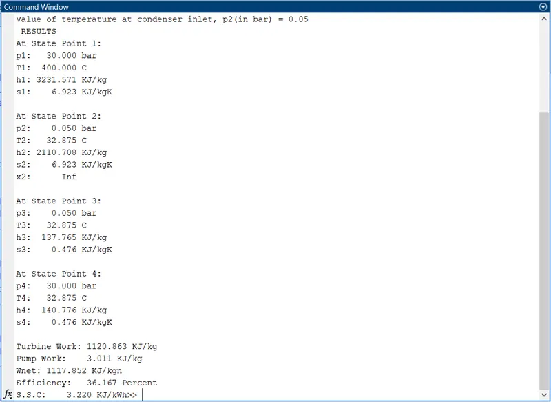
OUTPUT OF THE PROGRAM : Screenshots shared below of the output obtained.

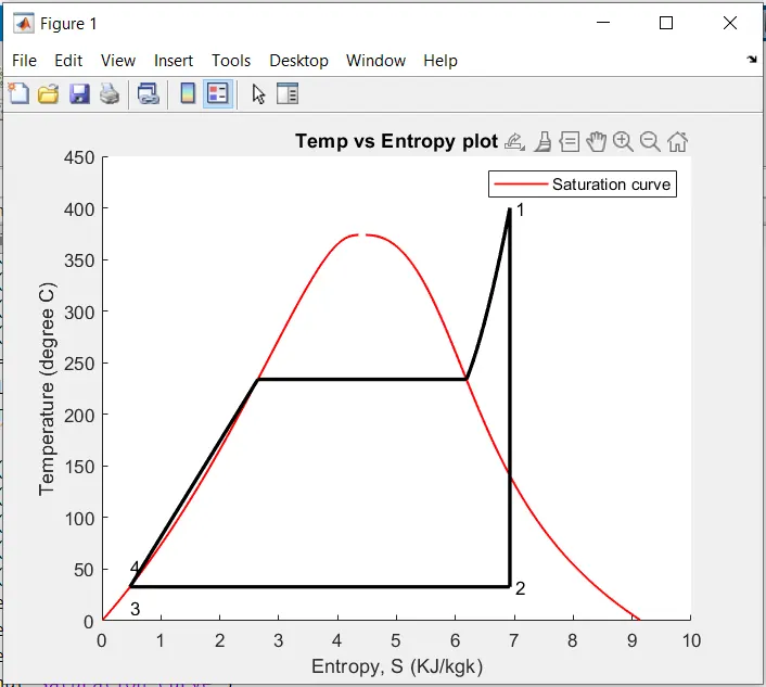
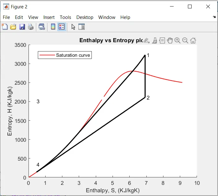
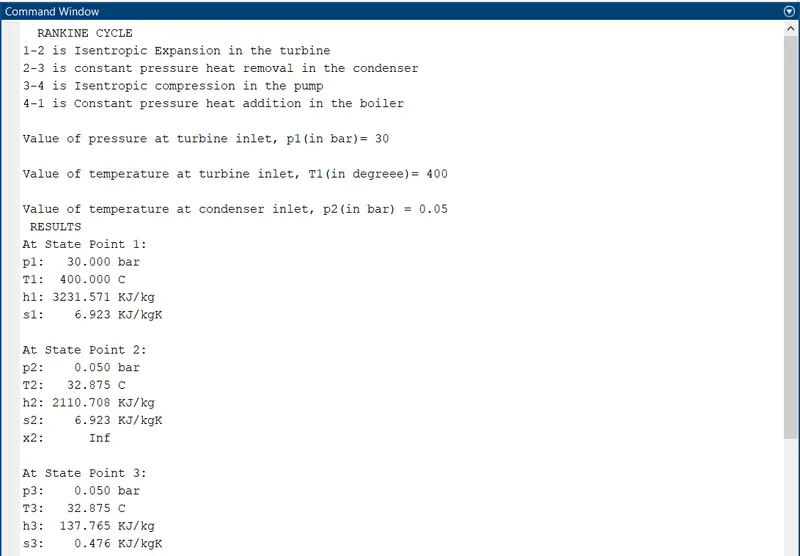
EXPLANATION OF THE PROGRAM:

1. XSteam data is used to extract steam and water properties of enthalpy, entropy at specific pressure and temperature for saturated liquid.
2. The program requires the input of Pressure (in bars) at state point 1(turbine inlet). Temperature at same point (in degree celcius) and Temperature at condenser inlet(point 2).
3. With the help of these inlets & from XSteam data, the program calculates all the state points of the Rankine cycle.
4. The XSteam data worked as:
5. h1 = XSteam('h_pT', p1, T1) : (returns the enthalpy of water at given pressure and temperature in bar and degree celcius respectively.)
6. As we extract data, we use thermodynamic relation to further find state points and extract their data from XSteam.
7. Sf, and sg,hf and hg, where f and g stands for saturated liquid and saturated vapour respectively .
8. The net work, work done by turbine, work done to run the pump. Heat in and heat out are calculated using standard thermodynamic relation.
9. Efficiency and Specific steam consumption (s.s.c) of the Rankine cycle is calculated.
10. T, s and h are extracted at vapour and liquid line for plotting purpose, after 4th point for the variation we observe in the plot.
11. Plot of T vs s and h vs s is created from all the points obtained from the program.
12. The plot changes as the user input changes for the above mentioned inputs.
13. Results are displayed in the command window.

There were a few errors I faced while programming. I have shared the screenshots of the errors thrown in the command window and also explained how i resolved them.

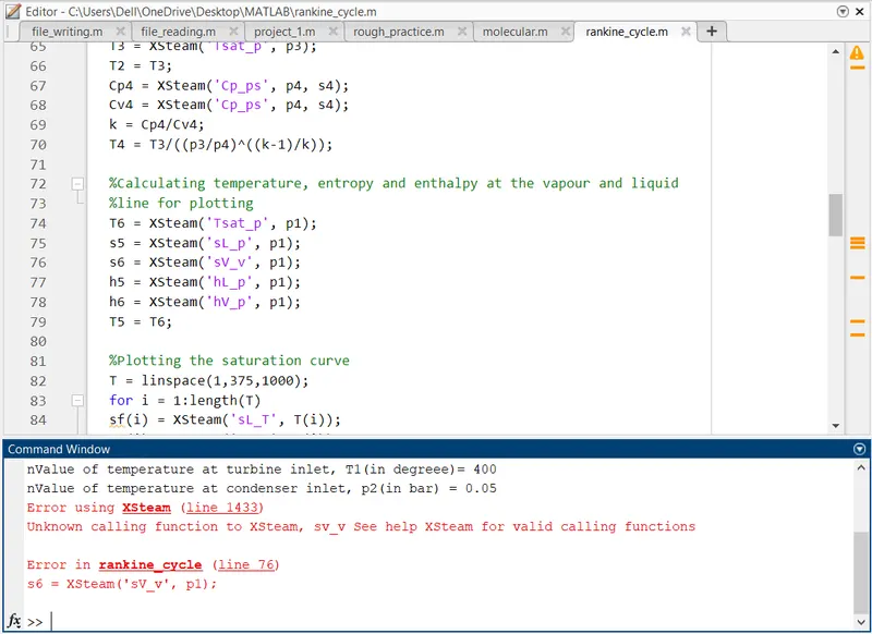
I got the above error because I coded 'sv_v' instead of 'sv_p'. (line 76). It was resolved by the coding accurately.

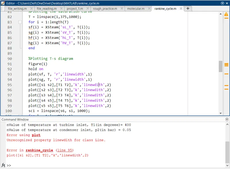
I got the above error because in line 95 I coded the spelling of the width incorrectly. It was resolved by coding correctly.

References :

1. https://en.wikipedia.org/wiki/Rankine-cycle
2. https://energyeducation.ca/encyclopedia/Rankine-cycle
3. https://in.mathswork.com/matlabcentral/fileexchange/9817-x-steam-thermodynamic-proerties-of-water-and-steam
4. https://www.youtube.com/watch?v=QFZN71MY710
5. https://www.sciencedirect.com/topics/earth-and-planetary-sciences/rankine-cycle