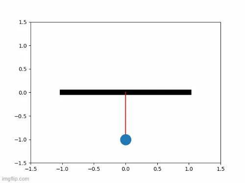
Week 3 - Solving second order ODEs

• AIM:

The main aim of the challenge is to write a program to solve ordinary differential equation of simple pendulum with damping using python.

• OBJECTIVE:

A simple pendulum consist of mass (m) attached by a string or rod of length(l) . When it is displaced to an initial angle and released, the pendulum will swingh back and forth with periodic motion.The figure shows the simple pendulum

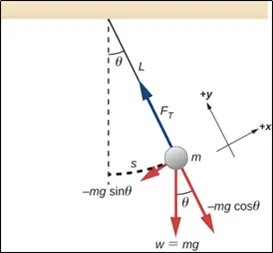
• GOVERNING EQUATION:

This equation represents the equation of motion of simple pendulum with damping.

`(d^2theta)/dt+b/m*(d theta)/dt+g/l*sin(theta)=0`

Breaking the governing equation;

say `theta = theta _1` .............(1) where b = damping coefficient

upon diffentiation w.r.t t we get, g = acceleration due to gravity in m/s^2

`(d theta)/dt = (d theta_1)/dt = theta_2`.......(2) l = length of rod in m

again upon diffentiation m = mass of bob in kg

`(d^2theta)/dt^2 = (d^2theta_1)/dt^2 = (d theta_2)/dt`...................(3)

from (2) and (3) we get

`(d theta_1)/dt = theta_2`

and `(d theta_2)/dt = -(b/m)*theta_2-(g/l)*sin(theta_1)`

• CODING:

import numpy as np
import math
import matplotlib.pyplot as plt
from scipy.integrate import odeint

#Function that returns dtheta/dt

def model(theta,t,b,g,l,m):
    theta1 = theta[0]
    theta2 = theta[1]
    dtheta1_dt = theta2
    dtheta2_dt = -(b/m)*theta2-(g/l)*math.sin(theta1)
    dtheta_dt = [dtheta1_dt,dtheta2_dt]
    return dtheta_dt

#Inputs
b = 0.05
g = 9.81
l = 1
m = 1

#Initial conditions
theta_0 = [0,3]

#Time array
t = np.linspace(0,20,200)

#Solving ordinary differential equation

theta = odeint(model,theta_0,t,args = (b,g,l,m))

#Plotting
plt.plot(t,theta[:,0],'g-',label='Angular displacement')
plt.plot(t,theta[:,1],'b--',label='Angular velocity')
plt.legend()
plt.xlabel('time')
plt.ylabel('Displacement&Velocity')
plt.show()

#Animation
ct = 1



for i in theta[:,0]:
    x0 = 0
    y0 = 0

    x1 = 1*math.sin(i)
    y1 = -1*math.cos(i)

    filename = 'test%05d.png'%ct
    ct = ct+1

    plt.figure()
    plt.plot([-1,1],[0,0],"black",linewidth=10)
    plt.plot([x0,x1],[y0,y1],"red")
    plt.plot(x1,y1,'o',markersize=20)
    plt.xlim([-1.5,1.5])
    plt.ylim([-1.5,1.5])
    plt.savefig(filename)

• EXPLANATION:

1. Import the required modules for the coding such as numpy,math and plot modules.
2. Enter the input values like damping coefficient,acceleration due to gravity,length of rod and mass of bob.
3. The governing equation is broken down to simple first order equation.
4. Enter the initial conditions such as displacement and velocity.
5. Create a function which returns the value of dtheta as theta varies.
6. odeint command is used to solve the ordinary differential equation.
7. Create a time array using linspace command.
8. Plot velocity and displacement againt time using plot command.

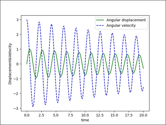
• PLOT:

• CONCLUSION:

We observe that if we increase damping coefficient system will returns to the equlibrium state faster and but overshoot one or more time.