Week 3 - Solving second order ODEs

1. Your objective is to write a program that solves the following ODE. This ODE represents the equation of motion of a simple pendulum with damping

Concept of Pendulum motion and its Dampening:

• The above equation given is the second-order form of a motion of a pendulum in damping.
• The given damping coefficient and other parameters are used as follows to reduce the equation into two first-order equations.

L=1 metre,

m=1 kg,

b=0.05.

g=9.81 m/s2.

let, `theta=theta_1`

`(d(theta))/dt=(d(theta_1))/dt=theta_2`............................................(1)

`(d^2(theta))/(dt^2)=(d^2(theta_1))/(dt^2)=(d(theta_2))/dt`.............(2)

From (1) and (2)

`(d(theta_1))/dt=theta_2` & `(d(theta_2))/dt=-(b/m)*theta_2-(g/l)sintheta_1`

Where,

`theta_1`= Angular Displacement

`theta_2`= Angular Velocity

Program for solving ODE representing the motion of simple pendulum with damping

%% Solving and Animating the damping of a Pendulum

%% Header
clear all 
close all
clc

%% Inputs
% Step1
l=1;        % length of pendulum
m=1;        % mass of the pendulum
b=0.05;     % damping coefficient
g=9.81;     % acceleration due to gravity

%% Initial conditions
% Step2
theta_0=[0;3];  % angular displacement and velocity at t=0s

%% Time of simulation
% Step3
t_animation=linspace(0,20,500); %time frame of the simulation

%% Solving ODE
% Step5
[t,results]=ode45(@(t,theta) ode_func(t,theta,b,g,l,m),t_animation,theta_0); % solving the differentioal equation using ODE54

%% Plots
% Step6
figure(1)
hold on
plot(t,results(:,1),'color','r')    % variation of displacement with time
plot(t,results(:,2),'color','b')    % variation of speed with time

xlabel('Time(s)')               % labelling x axis
ylabel('Plots')                 % labelling y axis
title('Damping of Pendulum')    % Title of the plot

%% Animation
% Step7
x = results(:,1);       % creating a new variable for displacement from results array

% Step8
ct=1;                   % counter variable to keep track of the plots as frames 
% Step9                   
for i=1:length(x)
    % Step10    
    x_1 = x(i);         % creating variable from displacement array
    
    % Creating points in x-y plane for the animation
    
    % Coordinate of the pendulum end points
    % Step11
    X0=0;               
    Y0=2;
    
    X1=l*sin(x_1);
    Y1=2-l*cos(x_1);
    
    X2= l*sin(x_1);
    Y2=2;
    
    X3=-l*sin(x_1);
    Y3=2;
    
    % Step12
    color=[0 0 0];      % RGB code of clolor black
       
    % Plots
    figure(2)
       
    % Step13
    plot([X0 X1],[Y0 Y1],[-0.5 0.5],[Y3 Y2],'linewidth',2)  % Making a plot from the coordinates
    hold on
    plot(X1,Y1,'-o','color',color)      % making the marker
    hold off
    axis([-1.3 1.4 0.7 2.2])            % for uniformity fixing the axis    
    title('Motion of Pendulum')         % title of the animation 
    pause(0.009)                        % To pause the code after the plot
    
    % Step14
    M(ct)=getframe(gcf);                % arranging the plot with counter
    ct=ct+1;                            % to make increasing counter pattern
end

% Step15
movie(M)            % used to play the frames stored in M
videofile=VideoWriter('Pendulum Animation.avi','Uncompressed AVI'); % Create object to write video files
open(videofile)             % Open file for writing video data
writeVideo(videofile,M)     % Write video data to file
close(videofile)            % Close file after writing video data
   

%% Function code for the Pendulum equation
% Step4(a)
function [dtheta_dt]=ode_func(t,theta,b,g,l,m)

% Step4(b)
theta1=theta(1);
theta2=theta(2);

% Step4(c)
dtheta1_dt=theta2;
dtheta2_dt=-(b/m)*theta2-(g/l)*sin(theta1);
dtheta_dt=[theta2;dtheta2_dt];
end

Explanation of Program

Step1:

• Input for the pendulum coefficients is given in this step.
• It includes the length of the pendulum(l), the mass of the bob(m), damping coefficient(b), and acceleration due to gravity(g).

Step2:

• To find the differential equation in solver ode45 the initial conditions are to provide which can be used to solve the equation.
• Here the inputs are in form of a column matrix of two rows where 1st row is angular displacement(`(theta_1)_0`) and 2nd row is the angular velocity(`(theta_2)_0`) at starting time(t=0).

Step3:

• As asked in the challenge we have to consider animating for 20 seconds.
• So a time array has been created between 0 to 20 with 500 elements in the array using syntax linspace.

Step4(a):

• Creating a function for the equation for the damping equation of the pendulum.
• The output of the function is [dtheta_dt], which is a column matrix of 2 elements.
• Inputs are t,theta,b,g,l,m respectively.

Step4(b):

• Defining the theta array for the solving of the second-order differential equation of the Pendulum in damping.
• The matrix is a row matrix that has two elements theta(1), and theta(2).

Step4(c):

• This step is for mentioning the equation for the solving of the damping equation of a simple pendulum.

Step5:

• The solver used is ode45 which is a medium order solver used to solve the differential equation.
• The syntax requires function variable(t,theta), then function inputs(t,theta,b,g,l,m) followed by the time span(t_animation) and then initial conditions(theta_0).
• The results from this solver are time span, input variables as results(theta1 and theta2 respectively). The results are formed as an array.

Step6:

• The solution of the above equation is printed in figure1 where we plot both angular displacement and velocity with damping in consideration.
• First, we plot the 1st column of the results array using the syntax(Results(:,1)) for the first column and syntax(Results(:,1)) for the second column.
• By using hold on command we can print both plots in one figure.
• To make the plot more informative a title, xlabel, and ylabel have been added to the figure.

Step7:

• For an animation of the pendulum, we started by making an angular displacement array(x) from the result matrix.

Step8:

• The counter(ct) is used to keep track of the plots as frames after each iteration of the loop, where we print the plot after each iteration.

Step9:

• A for loop is started where iteration(i) is defined from one to length(x).
• This means the loop runs for the 'i' number of times.

Step10:

• To use an element from x array we define another loop variable x_1 which also represents angular displacement corresponding to i.

Step11:

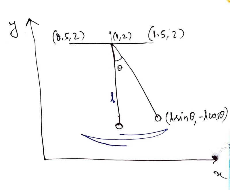
• This is the logic behind the animation, where we print the position of the pendulum for each x_1.
• This follows the above image.
• This has been used to create the coordinates of the pendulum.

Step12:

• A variable named color has been defined to store RGB color black to create a marker in the plot section.

Step13:

• The plot is saved in another plot window called figure2.
• The plotlines have been defined using plot syntax thereafter, for making the marker a hold on and hold off command is used to make the plot discrete.
• An axis has been defined to make sure all the iteration remains as a uniform plot using a syntax axis.
• A title is used to make the plot more meaningful and a pause command is used to make the plot stop to see it as a frame.

Step14:

• A variable M is defined to save the plot as a frame using getframe.
• The counter pattern is defined to store the frame in increasing order of the iteration.

Step15:

• movie(M) command is used to make a movie out of M where frames are saved in form of an array.
• A videofile has been made by using the command VideoWriter, where the video profile is also defined.
• The command open has been used to open the file and then command write is used to write all the frames of M in the videofile. Then close command is used to close the videofile.

Plot Results:

Plot for the damping:

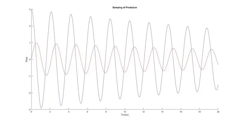
• Due to the low damping coefficient, the angular displacement is not being absorbed amplitude doesn't seem to reduce drastically.
• The same applies to angular velocity as well.
• The animation of Pendulum is given in the link below

https://youtu.be/cyixXh5yATo

Errors made along the way

• 
• This error happened due to the wrong brackets.
• 
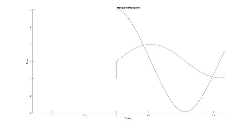
• This error plot is generated due to improper use of hold on.
• 
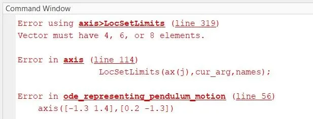
• This error occurred due to the wrong syntax for the axis after the plot of the animation.

Conclusion

I've tried to complete the challenge myself but was unable to finish without a small help from my Support engineer. The errors which I made throughout have taught me a lot. I hope I delivered the results properly. The printed plot is as expected from the problem.

All the files have been attached below.

Thank you.