Week 3 - Solving second order ODEs

SOLVING OSCILLATION OF A SINGLE PENDULUM USING SECOND ORDER ODE

1.AIM

To solve the equation on oscillation of a  single pendulum using second order  ODE and to make animation using python

2.OBJECTIVES

 write a program that solves the following ODE. This ODE represents the equation of motion of a simple pendulum .

Write a program in Python that will simulate the pendulum motion.

Simulate the motion between 0-20 sec, for angular displacement=0,angular velocity=3 rad/sec at time t=0.

2.GOVERNING EQUATIONS

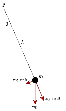
A simple pendulum consists of a ball (point-mass) hanging from a (massless) string of length L and fixed at a pivot point P. When displaced to an initial angle and released, the pendulum will swing back and forth with periodic motion. By applying Newton's second law for rotational systems, the equation of motion for the pendulum may be obtained.

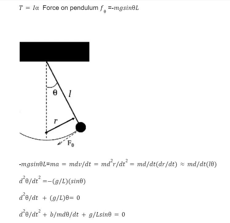
Where,

B-dambing , Damping is an influence within or upon an oscillatory system that has the effect of reducing or preventing its oscillation. To this end, the general assumption is that the drag force due to the air resistance on the bob of the pendulum is the cause of its damping, and normally the air resistance on the string of the pendulum is assumed to be negligibly small.

M-mass

g-gravity

L-length

a-acceleration due to gravity

ALGORITAM

Step1;start sublime text

Step2;import math. command is used to call trigonometric functions(mathematical function) and import matplotlib.pyplot as plt command to plot graphs in programing

Step3;numpy

Step4;odeint

step5;’equation ‘is a system/function that describes ordinary differential equations which consists of inputs of initial variables mass,length,time ,damping coefficients and acceleration due to gravity

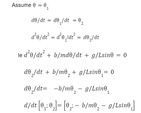
Step6; theta of 0 [first differential] is assigned to a variable  theta 1 and theta of [1] [second order differential]  is assigned to a variable name theta2

Step7; first order differential of   gives  displacement which is 

Step8;first order differential of   gives velocity given by the equation   

Step9;assign as a column matrix of  and  ,where  is initial displacement and  is initial velocity

step10; command return theta will give each value of theta

step11; input value of mass,length,time ,damping coefficients and acceleration due to gravity

Step12;initial disp and velocity given and assigned to theta_0

step13;linspace is a command used to make 150 values between 0 to 10 t=np.linspace(0,10,150),time period of oscillation given by linspace command

step15;odeint is a command used to solve ordinary differential equations .odeint a function to integrate a system  of ordinary differential equation.To pass the ode integral we need to iput(ode,initial conditions,time,arguments)

step16;plt.plot(t,theta[:,0],'b-',label=angular displacement') first column gives displacement.

            plt.plot(t,theta[:,1],'r--',label=velocity')second column gives velocity

Step17;label the plot using plt.label command wrt to time

Step18;put legends ,plt.show command to plot graph

ANIMATION OF PENDULUM

Step19;contour initialized

Step20;x0,yo marked started from 0

step21;for t in displacement x and y increment given by equation   

 x1=x0+(1*math.sin(t))

 y1=y0-(1*math.cos(t))

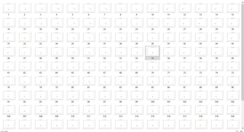
step23;save as string in png format and  give file name

Step24,contour increased using ct=ct+1

Step12;plt figure command to plot the graph

Step13;plot commands plt.plot([x0,x1],[y0,y1]) to plot bob with size20 using marker size command. plt.plot(x1 toy1)

step14; x limits and y limits are given to set axis

Step15;save the figure using save command

Step16;end the program

#animation of simple pendulum 
#second order ODE
import numpy as np 
from scipy.integrate import  odeint
import matplotlib.pyplot as plt
import math
#equation is system that describes ordinary differention equations
def equation(theta,t ,b,g,l,m):
	theta1=theta[0]
	theta2=theta[1]
	#defining ordinary equations
	dtheta1_dt=theta2
	dtheta2_dt=-(b/m)*theta2-(g/l)*math.sin(theta1)
	dtheta_dt=[dtheta1_dt,dtheta2_dt]
	return dtheta_dt 

b=0.02
g=9.81
l=1
m=0.1
#theta_0=[disp,velocity}
theta_0=[0,3]
#linspace is a command used to make 150 values between 0 to 10
t=np.linspace(0,20,150)
#odeint is a command used to solve ordinary differential equations
#odeint a function to integrate a system  of ordinary differential equation
#To pass the odeintegral we need to iput(ode,initial conditions,time,arguments)
theta=odeint(equation,theta_0,t,args=(b,g,l,m))
#print(t)

#print(theta)

plt.plot(t,theta[:,0],'b-',label=r'angular displacement')
plt.plot(t,theta[:,1],'r--',label=r'velocity')
plt.ylabel('plot')
plt.xlabel('time')
plt.legend(loc='best')
plt.show()

ct=1
x0=0
y0=0
for y in  theta[:,0]:
     x1=x0+(l*math.sin(y))
     y1=y0-(l*math.cos(y))
     

     filename=str(ct)+'.png' 
     
     plt.figure()
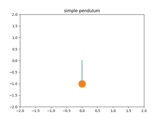
     plt.plot([x0,x1],[y0,y1])
     plt.plot(x1,y1,'o',markersize=20)
     plt.xlim([-2,2])
     plt.ylim([-2,2])
     plt.title('simple pendulum')
     plt.savefig(filename)
     ct=ct+1

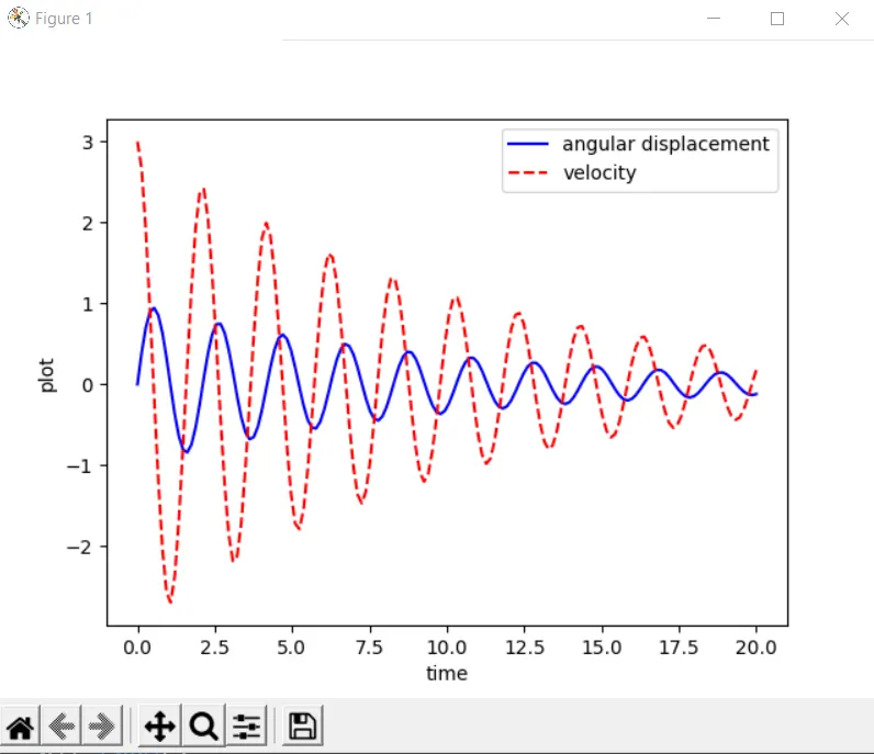
OUTPUT

CONCLUSION

The python program to make an animation of a pendulum has been executed successfully and the output is verified.