Week 3 - Pitot tube

Aim: A pitot static tube

a.You are required to do a literature review of pitot-static tube. Also establish a relationship between Total (stagnation) pressure and static pressure

b.You are required to create surfaces and fill it separately for Total pressure port and static pressure port

2. For the values of velocity given below calculate the total and static pressures and find the error in percentage for velocity.

Velocity(m/s)	Gauge Pressure (Pa)
240	-2817
100	33287
62	65780

Pitot Tube Theory:

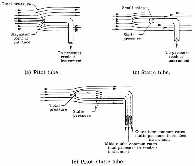
• A pitot tube or a pitot probe is a flow measurement appliance used to calculate the fluid flow velocity. French engineer Henri Pitot invented the pitot tube in the early 18th century. In the mid-19th century, French scientist Henry Darcy altered it to its modern form.
• Pitot tubes are widely utilised to determine a boat’s water speed, the airspeed of an aircraft, and measure air, liquid and gas flow velocities in various industrial applications.

Working Principle:

• Static Pressure is the pressure excerted by the fluid due to random motion of the molecule. Gauge pressure is the pressure measured by the instrument with respect to the atmospheric pressure. Absolute pressure is the sum of atmospheric pressure and gauge pressure.
• Lets us consider the pitot static tube, the tube is place in the flowing fluid for which the velocity is to be measured.

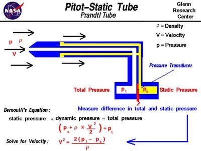
• The central tube initially allows the fluid to flow as there is no outlet, the fluid gets accumulated and the velocity of the fluid becomes zero or stagnation velocity is zero. Corresponding pressure is known as the Total pressure.
• There is another outer tube which has opening perpendicular to the flow field which measures the static pressure of the fluid.
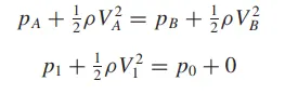
• Now, by using the Bernoulli’s equation. In particular, apply Bernoulli’s equation between point A, where the pressure and velocity are P1 and V1, respectively, and point B, where the pressure and velocity are P0 and V = 0, respectively

now,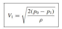

• So by finding the static pressure (P1) and Total Pressure (P0), we could find the velocity of the flowing fluid at low mach number.

Setup:

• The given mesh model is imported to the fluent mesh, and then the setup file is changed accordingly.

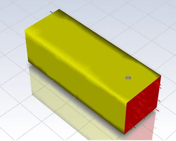
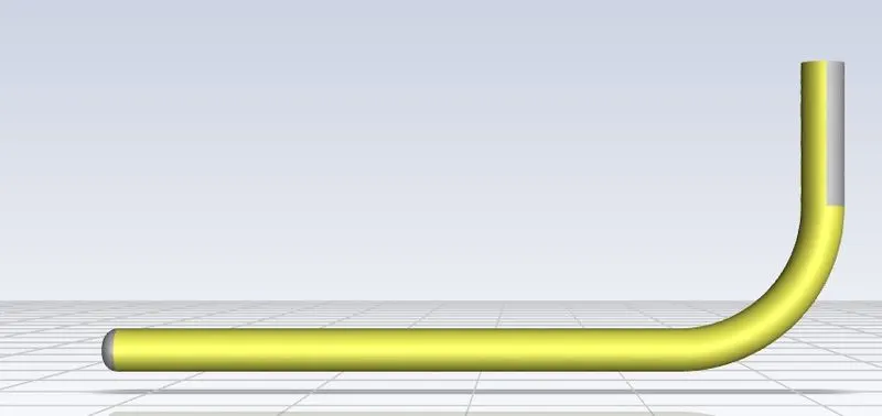
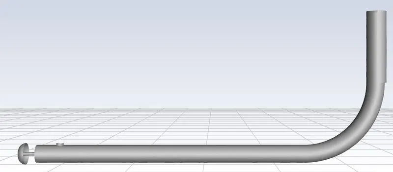
• Here, we choose the flow to be incompressible and steady laminar flow hence choosed pressure based solver with laminar model. The working fluid is considered to be Air.

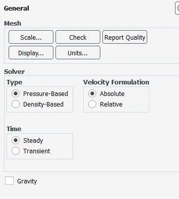
• As the flow is incompressible and the density of the fluid is assumed to be constant, the operating pressure is of least importance. Even if we use the operating pressure to be 101325Pa the result will be similar only.

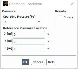
• Set the inlet and Outlet Boundary condition according to the case you are simulating.

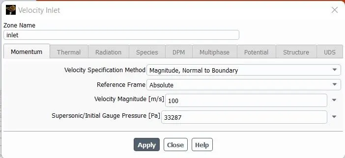
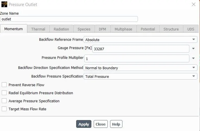
• Create a point probe near the outer tube & inner tube to measure the pressure.

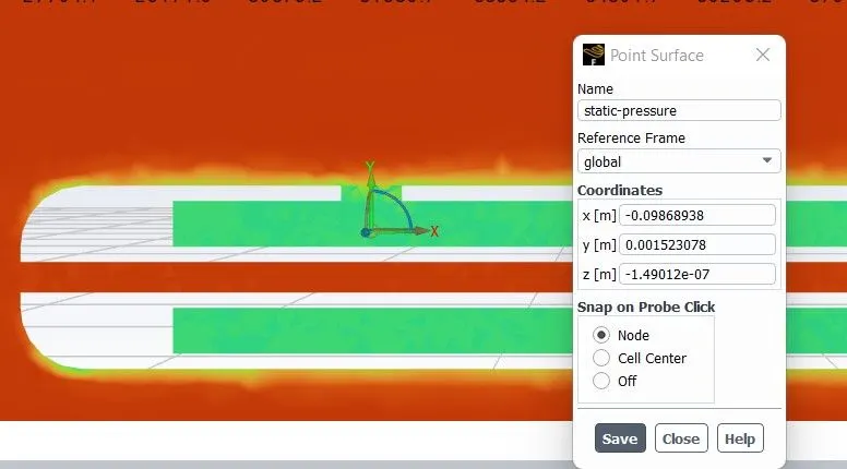
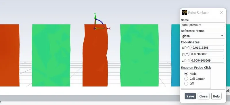
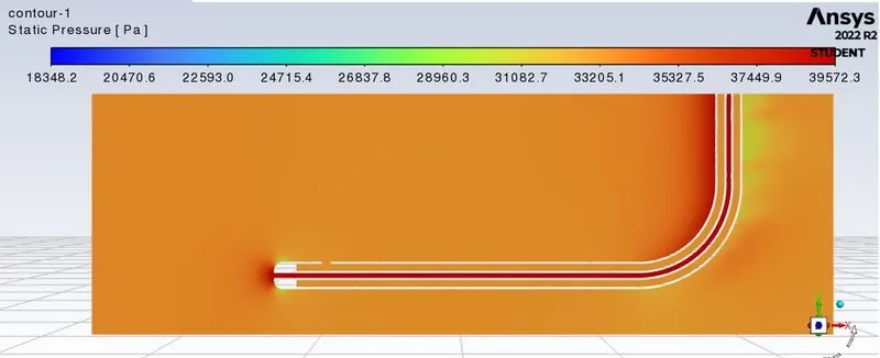
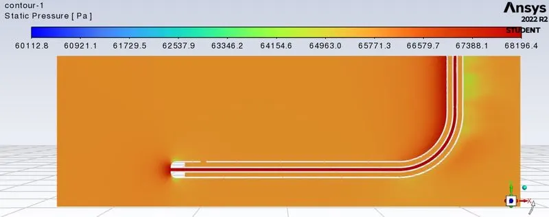
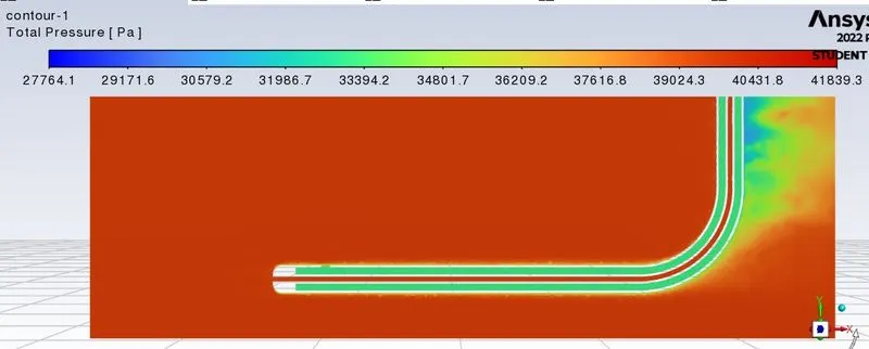
• Using the point probe find the Area weighted average for static pressure, total pressure accordingly. Create a report for the area weighted average for outlet surface.

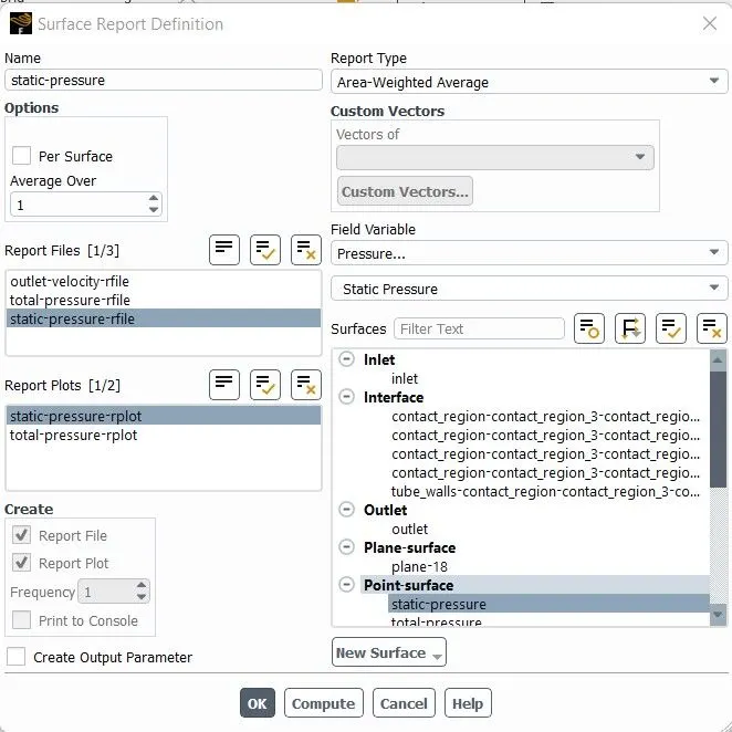
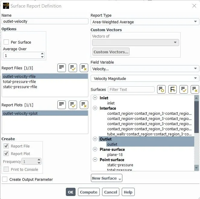
Output:

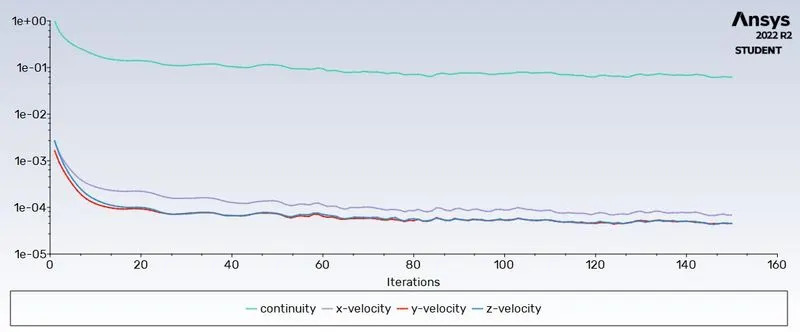
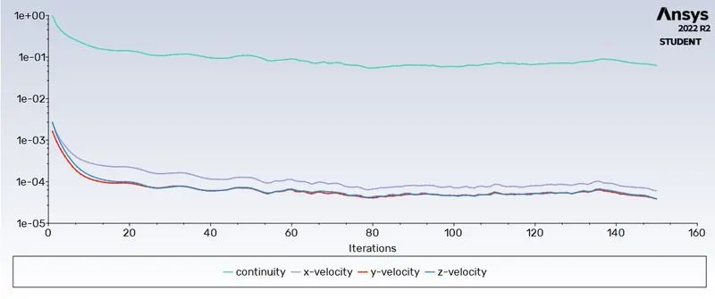
Parameters	Case 1	Case 2	Case 3
Inlet Velocity (m/s)	240	100	62
Inlet & Outlet Gauge Pressure (Pa)	-2817	33287	65780
Residual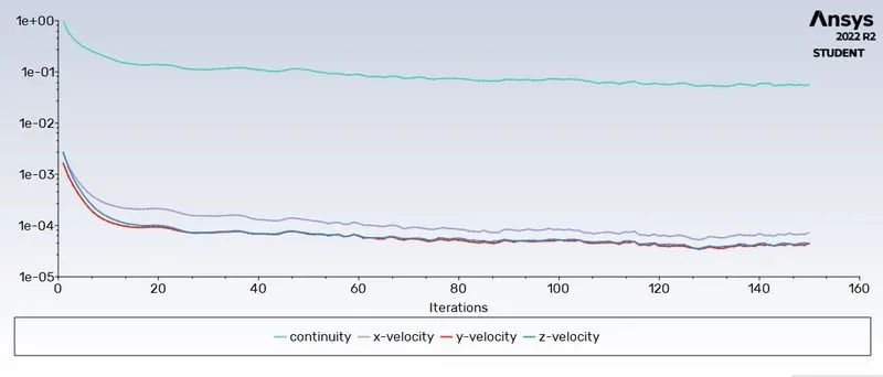
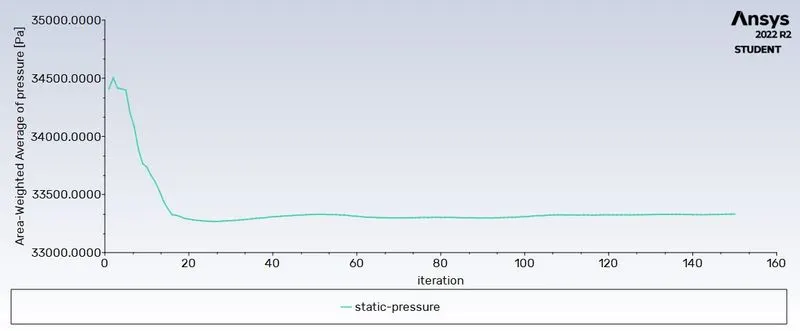
Static Pressure Plot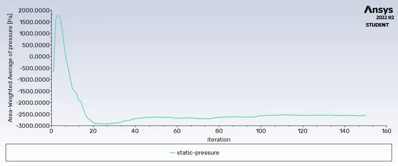
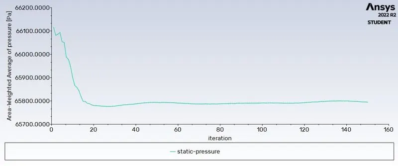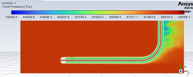
Total Pressure Plot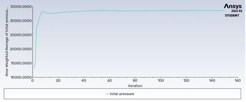
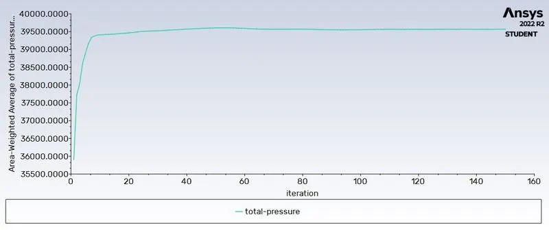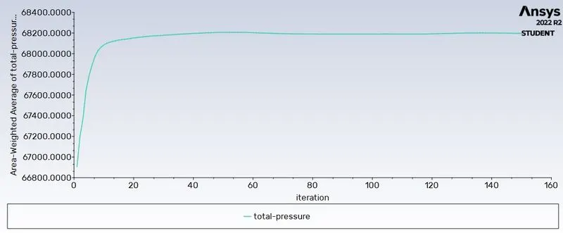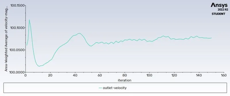
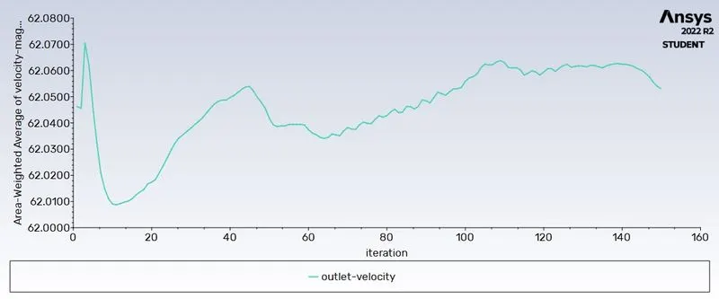
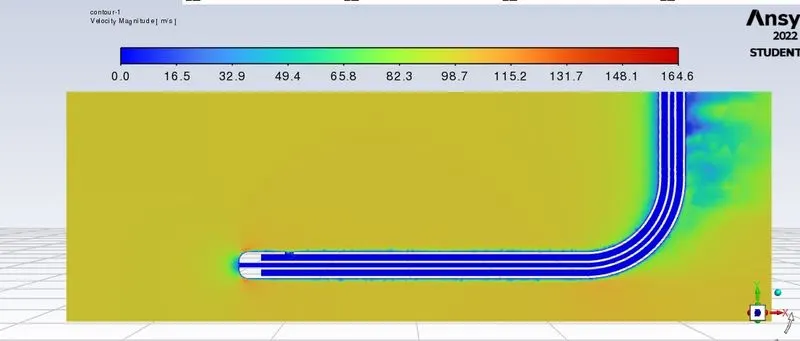
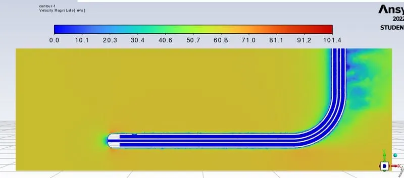
Outlet Velocity Plot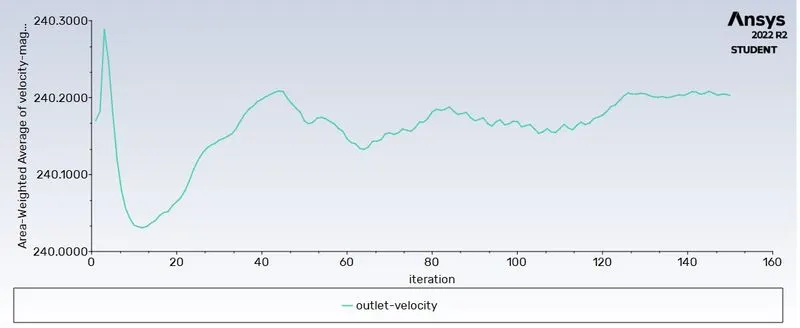
Static Pressure Contour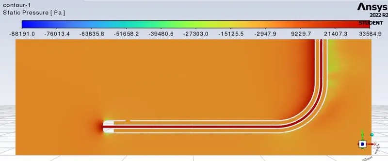
Total Pressure Contour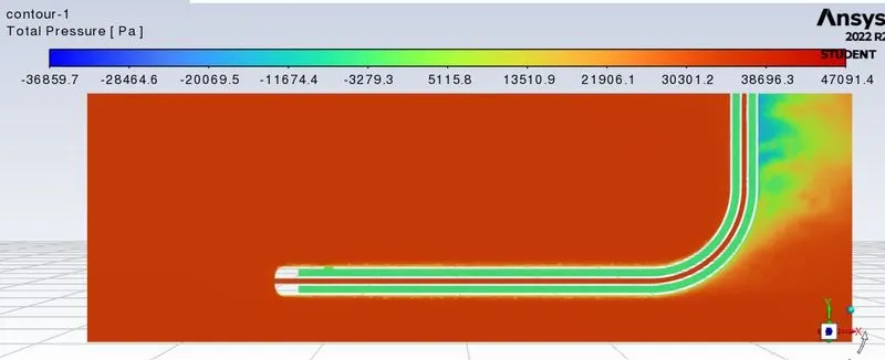
Velocity Contour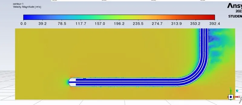
Result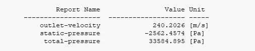

Calculation:

For, case-1

velocity `V=sqrt(((Po-Ps)*2)/rho)=sqrt(((33584.895-(-2562.4574))*2)/1.225)=242.932m/s`

% Error =`abs(Vs-Va)/(Va)*100=abs(242.932-240)/(240)*100=1.22%`

Result:

Case Study	Actual Velocity (m/s)	Static Pressure (Pa)	Total Pressure (Pa)	Simulation Velocity (m/s)	% Error
1	240	-2562.4574	33584.895	242.932	1.22
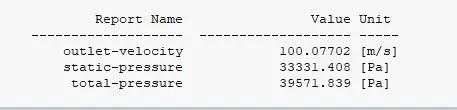
2	100	33331.408	39571.839	100.938	0.94
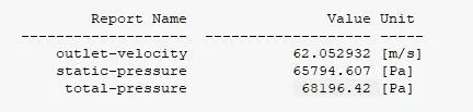
3	62	65794.607	68196.42	62.621	1.00

Conclusion:

• Thus, the flow simulation for different Velocity & Pressure is simulated.
• Velocity obtained from the simulation is within the acceptable limit (i.e. less than 5% Error).