Week 3 - Pitot tube
Pitot static tube
In the world of aeronautics it is often observed that to understand the velocity of the flow or to know at what velocity the aircraft is moving, pressure difference is employed. Not for the lack of sensing equipmesnt but the pressure difference with the density of the fluid at a certain height is a pretty good way to calculate the velocity of the object. In this process a relationship is established between total pressure, static pressure and dynamic pressure. A device used to acertain the static and dynamic pressure is a pitot tube.
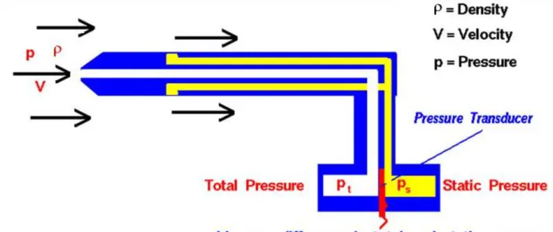 |
The working of tis device doen not involve any mechanical part and it take data directly from the flow and makes calculations. The bore facing the flow is used to calculate the total pressure and the bore perpendicular to the flow calculates the static pressure. With this information and using the formula:
Total pressure = Static pressure + Dynamic pressure.
where,
Dynamic pressure = `1/2 * rho * v^2`
By manipulating the equatio based on the values known,
we can write,
`v^2 = (2*(P(t) - P(s)))/rho`
This equation gives the velocity of the flow/object.
Simulation conducted with three cases, is given below:
|
Case |
Velocity(m/s) |
Gauge Pressure (Pa) |
|
1 |
240 |
-2817 |
|
2 |
100 |
33287 |
|
3 |
62 |
65780 |
Usinf these values we can simulate the flow over Pitot tube.
The following is the case setup,
Viscous model: Laminar
Material Properties: Density : 0.863 `(kg)/(m^3)`
Viscosity : 1.678e-5 `(kg)/(m-s)`
Boundary conditions: Depends on the case for velocity and pressure. (Pressure will be put in both inlet and outlet)
Operating pressure: 0 Pa
Simulation result:
|
Case 1
|
||
|
Case 2
|
||
|
Case 3
|
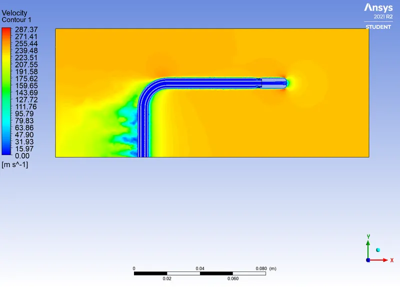
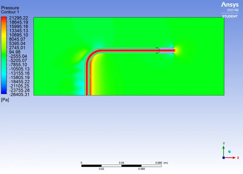
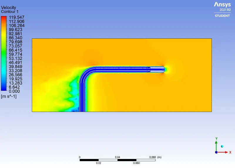
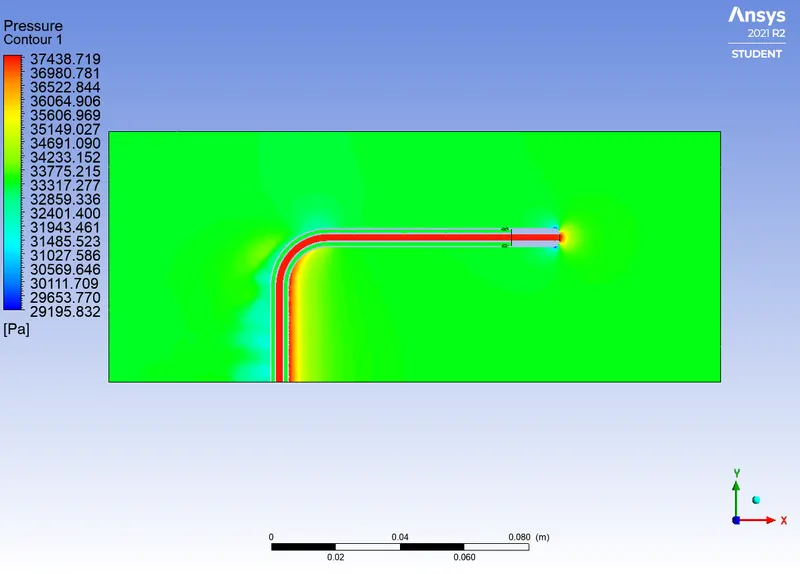
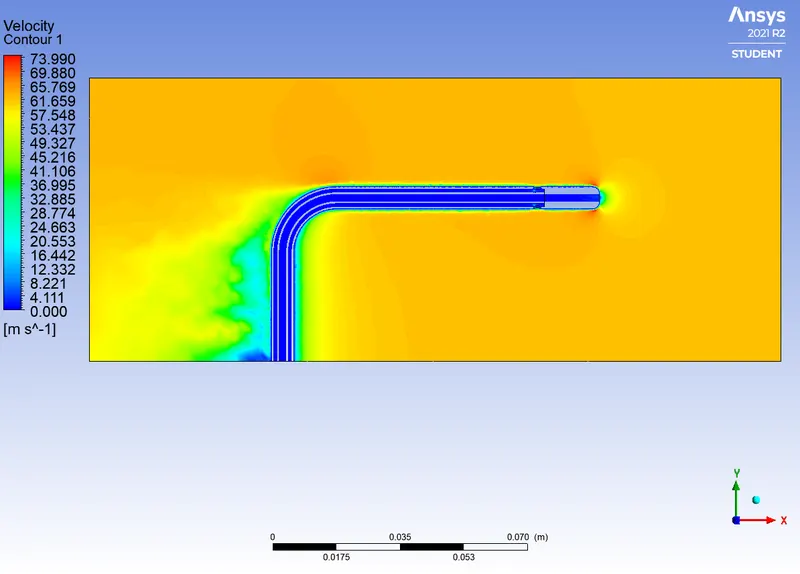
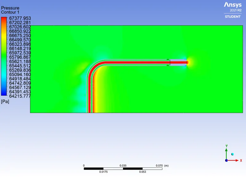
| Velocity GIVEN | 240 m/s | 100 m/s | 62 m/s |
| Total pressure | 21453.202 Pa | 33298.841 Pa | 67382.905 Pa |
| Static pressure | 2621.668 Pa | 37431.635 Pa | 65782.742 Pa |
| Velocity obtained | 236.2 m/s | 97.86 m/s | 60.89 m/s |
| Error % | 1.60% | 2.18% | 1.822% |
Conclusion: In this study we tried to understand the woriing of a Pitot tube. Using the given cases and validating the values analyticall ywe can observe theerror percentage is between 1-2% which is appriciable. Hence, we can conclude the simulation is conducted successfully.