Week 3: Flow over a backward facing step

Aim: Simulating flow over backward facing step.

Objective:

1. Create a backward facing step geometry in converge.
2. Set a case and simulate for three different base mesh sizes:

• dx = dy = dz =2e-3m
• dx = dy = dz =1.5e-3m
• dx = dy = dz =1.0e-3m

Introduction:

Many industrial application involves flow seperation and reattachment, the backward facing step is one where we discuss such phenomenon and the effect due to which flow seperation takes place.

In our simulation the fully developed flow enters the domain from left. When the air or the fluid used reaches the step, because of pressure gradient the expansion in flow occurs which causes it to detach and form a recirculation zone.

Seperation and reattachment of turbulent flow occur in many practical applications ex: combusters, diffusers , flow around airfoil and building.

The major reason for flow seperation is adverse pressure gradient which is due to increase in static pressure in flow direction. this causes increase in potential energy and decrease in kinetic energy and slowing down a fluid which causes its seperation from wall.

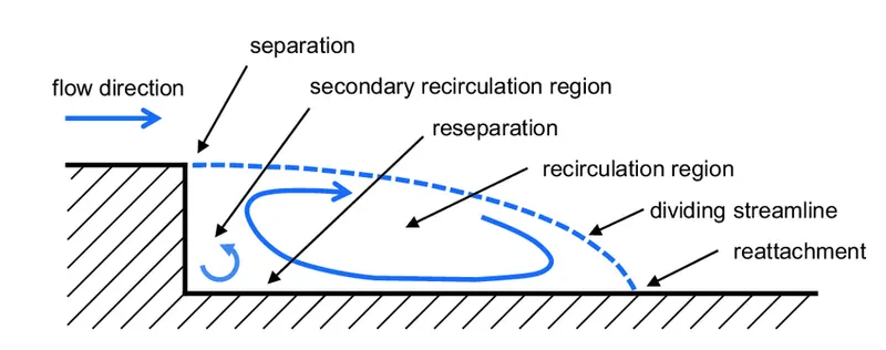
In the above image we can find out all the major regions present in backward facing step flow.

We can create the geometry in Converge CFD software or any modelling software and import it.

Steps to create a geometry in Converge CFD:

Step 1: Create a vertices for all points which defines the shapes.

Step 2: Using create triangle using vertices options create triangles and we are done with 2d shape.

Step 3: We can copy same shape at some offset and use loft edges option we get the finished 3-d shape or we can use sweep option and sweep the shape upto a required thickness and then use patch to cover the uncovered side.

Backward facing step geometry:

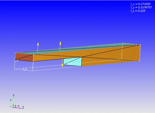
Once the geometry is created running the diagnosis is must to check if there is any error in geometry once there are no error we can proceed for setting up the case.

• Select the required dialog box for all the parameters that appear in the case of the setup tree, once selected we can start adding on the values i.e.

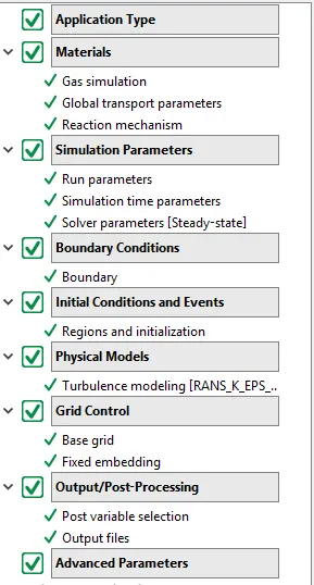
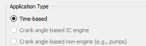
• The first parameter is application type which should be selected as à time base (since we are simulating steady-state simulation)

• The next parameters are materials in which we should check the following dialog boxes , gas simulation, global transport properties, and reaction mechanism. For gas simulation, and transport properties we should keep the properties as same.
• Now we add values for simulation parameters in which we should check the following dialog boxes run parameter, simulation time parameters, and solver parameters.

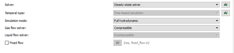
• In simulation parameters, we can control start time-end time and time steps also CFL number which actually controls the stability of any solution.

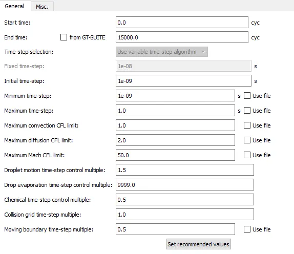
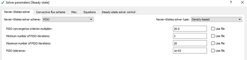
• In solver parameters, we will specify the solver scheme and can make choice in b/w density-based or pressure-based solver type.

• It’s Turn to add boundary condition the five boundaries are being named as an inflow (inlet), Outflow (outlet), TWO_D (Front and back), and the wall (top and bottom).
• Now it is a turn to provide a volumetric region on which initial conditions can be applied which can be set inside initial conditions and events in regions and initialization.

The pressure value for the volumetric region is 1 bar and temperature 300k

• We will be using turbulence modelling for this case.
• The next step is to add a grid which can be done in Grid control à base grid.

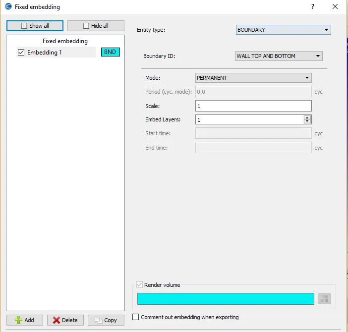
Three different base mesh sizes are being added and we will be using fixed embedding at boundsry of the shape.

The fixed embedding is used when we require a finer mesh elements at boundary of the geometry to get a accurate results at the boundaries.

• The final step in case set-up is Output/Post-processing in this section we can define the time interval for writing a 3D – output file such that we can get a maximum number of post-processed files for smooth animation.

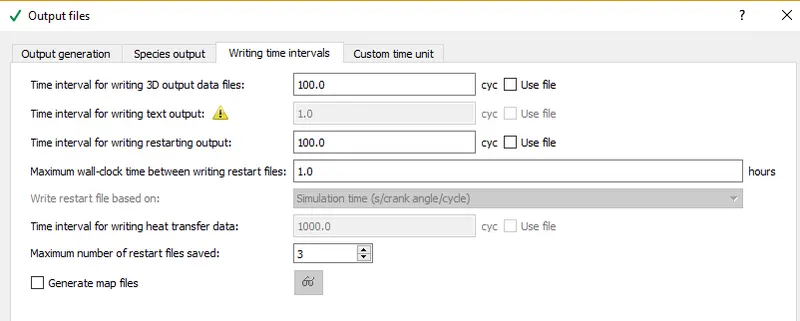
Step 4: Saving all the input files in a single folder, and copy the mpiexec.exe file to the folder.

Step 5: Running the simulation using Cygwin.

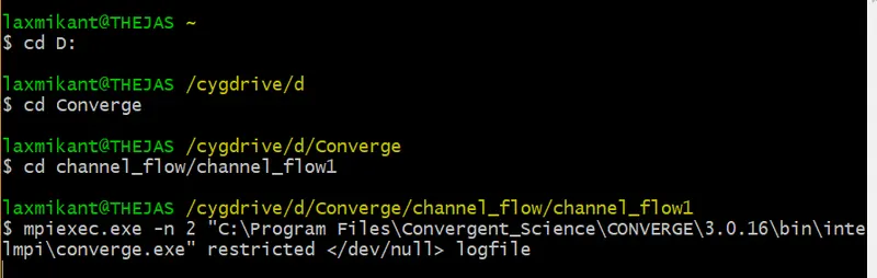
Step 6: Post-processing in Converge in Vtk binary inline format.

Step 7: Visualizing the case in ParaView also saving the animation, contours, and plots.

Mesh for all three base cases:

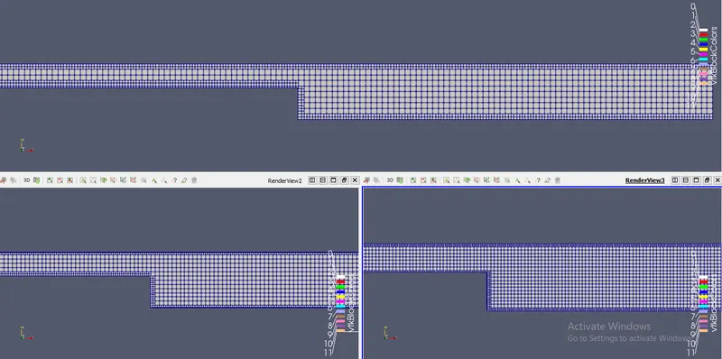
From above image the difference can be seen in mesh grids by counting the number of cells at particular location.

Case 1:

• dx = dy = dz =2e-3m

Converge plots for mass flow rate, average velocity and cell count:

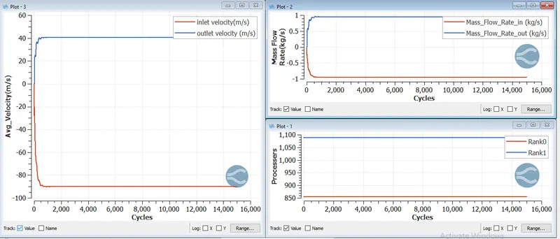
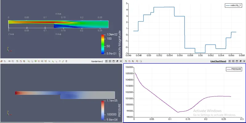
Velocity contour and pressure contour at final time step:

Case 2:

• dx = dy = dz =1.5e-3m

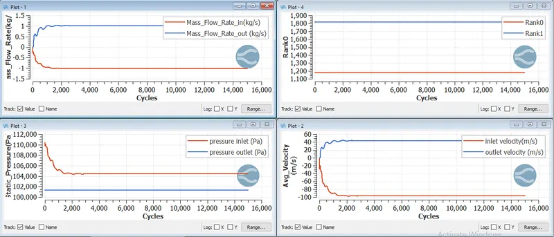
Converge plots for mass flow rate, average velocity and cell count:

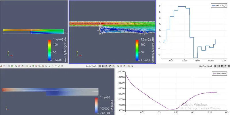
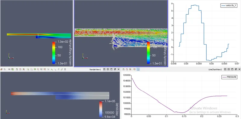
Velocity contour, pressure contour, and gylph at final time step:

Case 3:

• dx = dy = dz =1e-3m

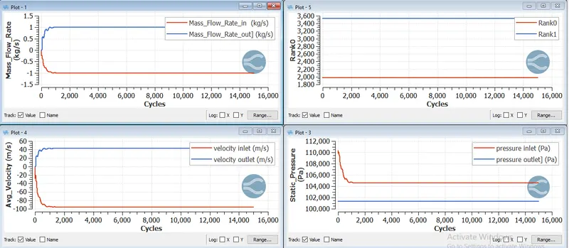
Converge plots for mass flow rate, average velocity and cell count:

Velocity contour, pressure contour, and gylph at final time step:

Link of animation for mesh size 1e-3:

https://drive.google.com/file/d/1U2yWNZ-vop3Fpc67Sw0gVDjleKZ0Hd6Y/view?usp=sharing

Conclusions:

• From above simulation we can say that as mesh becomes more finer the cell count increases and also the accuracy of the solution.
• In backward facing step we find a flow seperation which takes place as the static pressure increases due to sudden expansion in flow.
• Due to recirculation the eddies are formed in empty space below the flow streamline which turns the laminar flow into turbulent flow.
• If we use fillet instead of using sharp corner we can avoid the flow seperation which in turn will increase the velocity and decrease the noise in the system.
• The pressure in a backward facing step first goes on decreasing reach a minimum where sudden expansion takes place and then increases before leaving the system, the pessure decreases because of change in volume.
• The velocity is maximum and fully developed at upper portion of geometry and minimum at lower end because of flow seperation which produces a gap beneath streamline.