Week 3: Flow over a backward facing step
Aim
- To simulate an airflow through a backward facing step using converge
- Simulate through three different cases by changing only mesh size
- Show the mesh of each cases
- Post-process the results and obtain pressure and velocity contours
- To plot mass flow rate, Velocity and pressure
Why separation is taking place
When a fluid flows around a body, forces act between the fluid and the surface due to the viscosity. These intermolecular forces are the caue for the drag, among other things. However, due to the forces acting, the surface of the solid body also tries to bind the fluid to itself. This also leads to the fluid adhering to the surface (no-slip condition). The layer above this adherent fluid layer will not be able to simply tear itself away from it, because intermolecular attraction and pressure forces also act between the layers. As a result, any flow flowing around a body is tempted to follow the profile of the surface.
In the case of sharp transitions or when flowing around blunt bodies, however, the fluid is often no longer able to follow the profile. The boundary layer or flow begins to detach itself from the body surface. This is referred to as a boundary layer separation or flow separation. Downstream of the separation point, vortices often form, resulting in a turbulent flow. A flow separation is particularly dangerous on the wings of an aircraft, as this also causes a loss of lift and the aircraft is in danger of crashing. In aviation such a dangerous flow separation is called stall.
Problem Definition
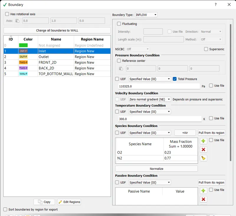
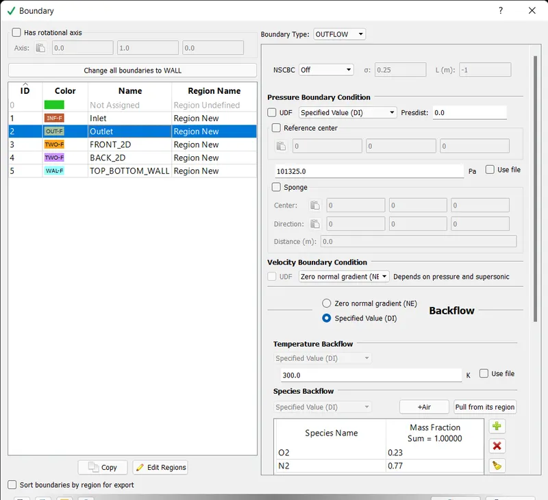
- Inlet pressure = 110325 pa
- Outlet pressure = 101325 pa
- Mesh sizes to be simulated - 2e-3,1.5e-3 and 1e-3
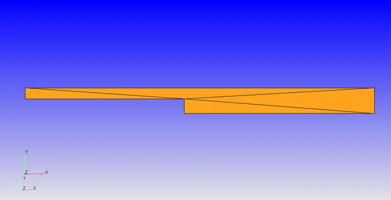
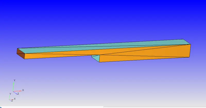
Boundary layer seperation
Setup
- Time based simulation is set
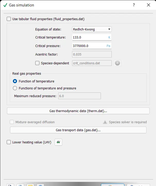
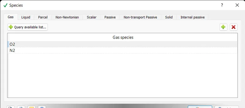
- Material is set to air contains 0.77 of nitrogen and 0.23 of oxygen also species involvemnt is also enabled
- species are added accordingly
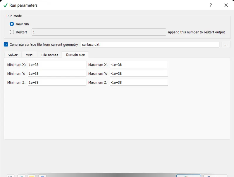
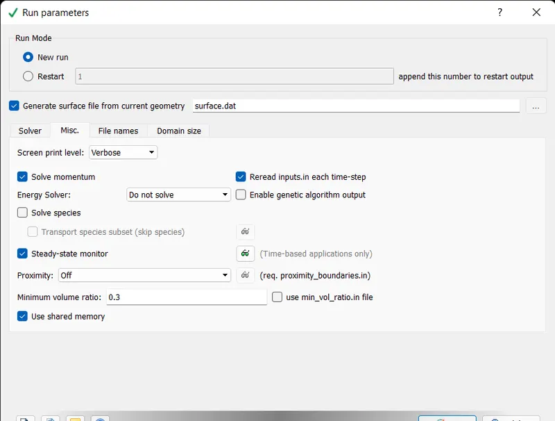
- In run parameters enregy involvement is disabled as we dont want temperature analysis
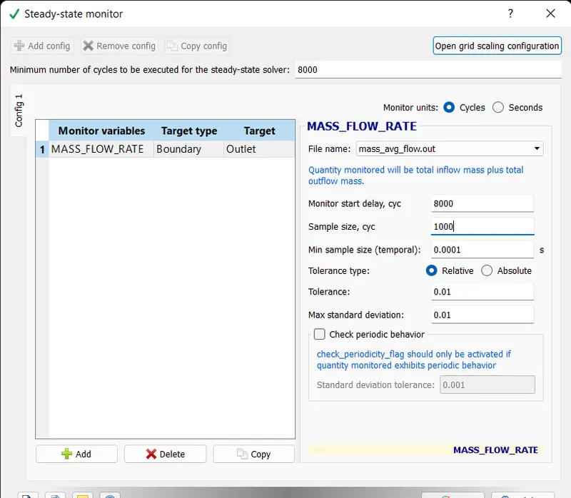
- Steady state monitor is turned on
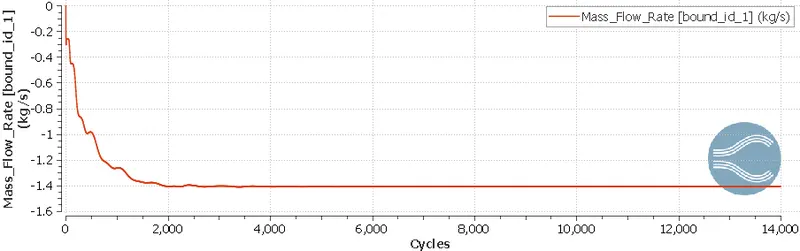
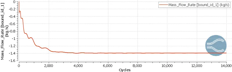
- Under steady state monitor mass flow rate is selected to check the convergency of the solution with sample size is set to 1000 and monitor start delay to 8000. Minimum cycles to be executed is set to 8000
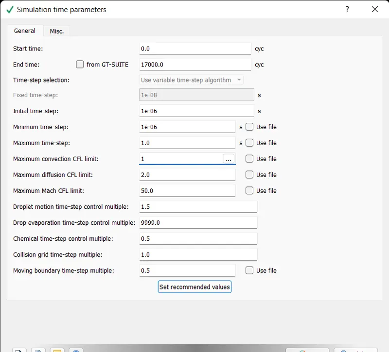
- Under simulation time parameter cycles to be executed is set from 0 to 17000,initial and minimum time step is set to 1e-6 whereas the maximum time step is to 1. The maximum CFL for convection is set to 1
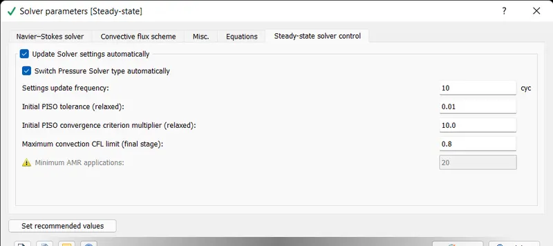
- Under solver paramteres,under steady state solver the maximum CFL limit of convection is set to a value less than 1 which is 0.8 inorder to avoid the chances of divergance
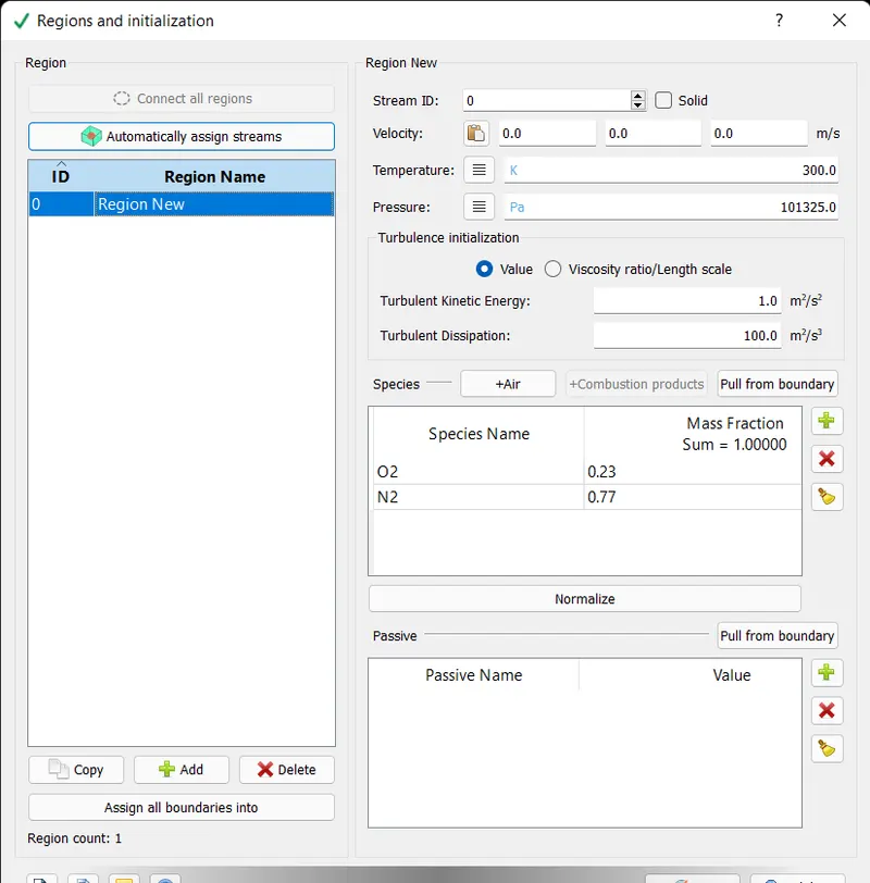
- A new region containing air is created in 'region and initialisation' and the initial pressure is set to 101325 pa
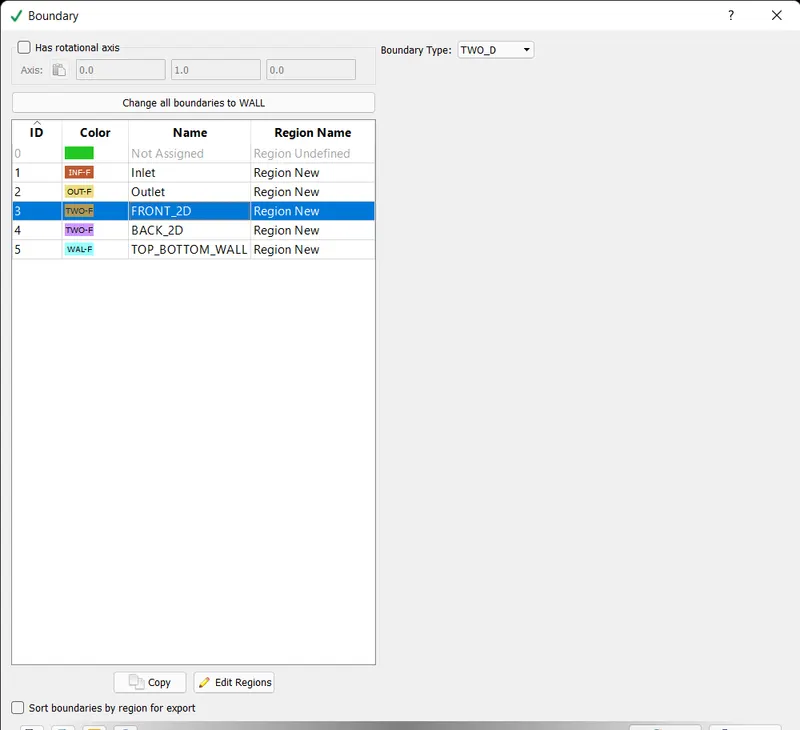
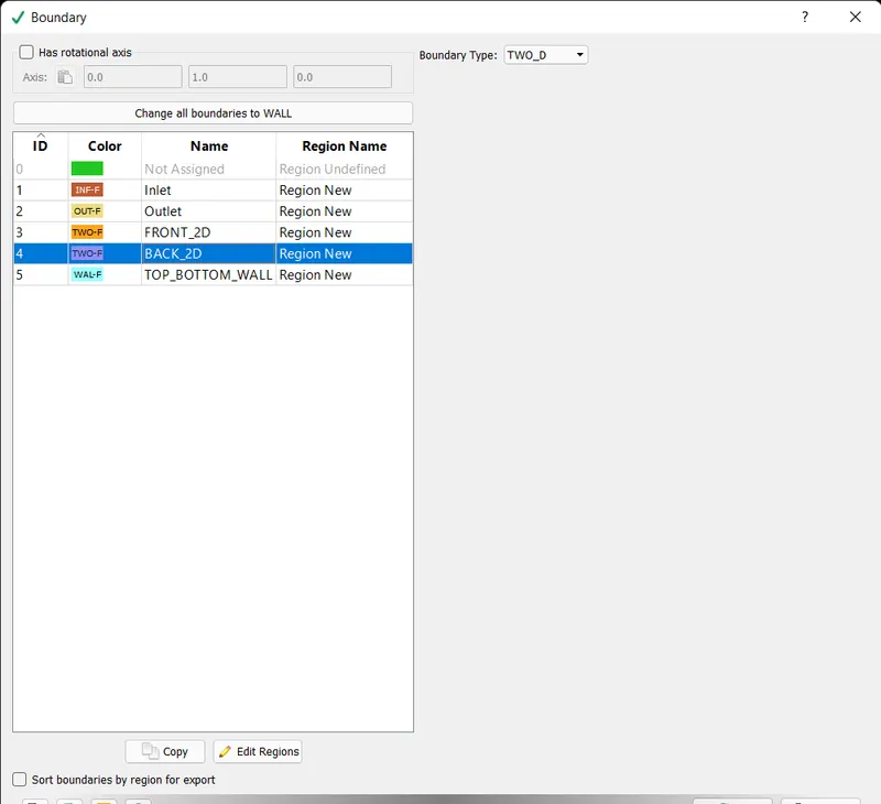
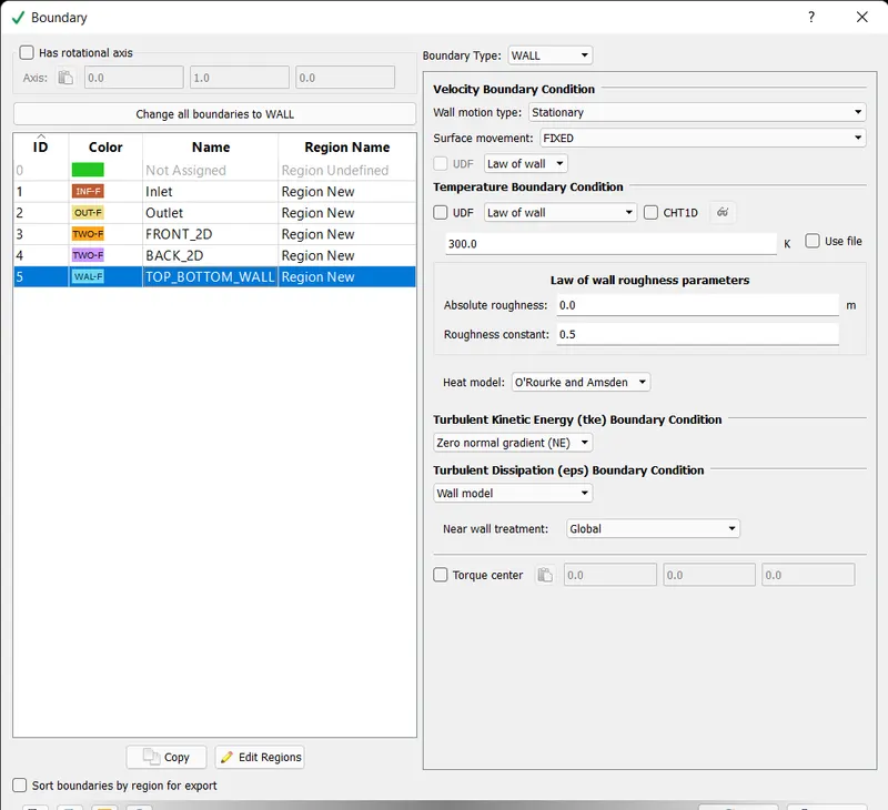
- Boundary conditions are set and shown the screen shots
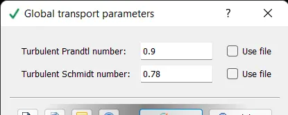
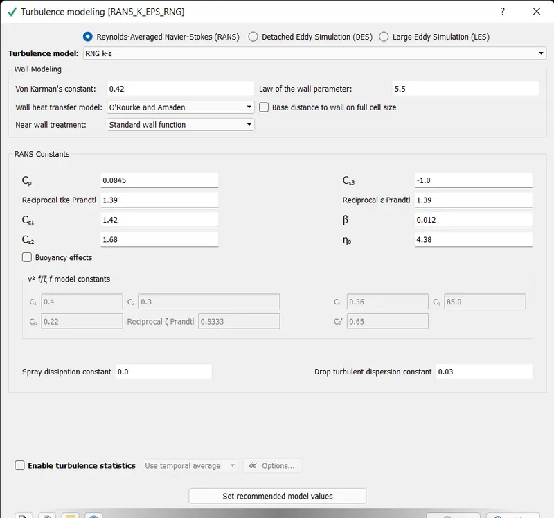
- RANS model is selected under turbulance model
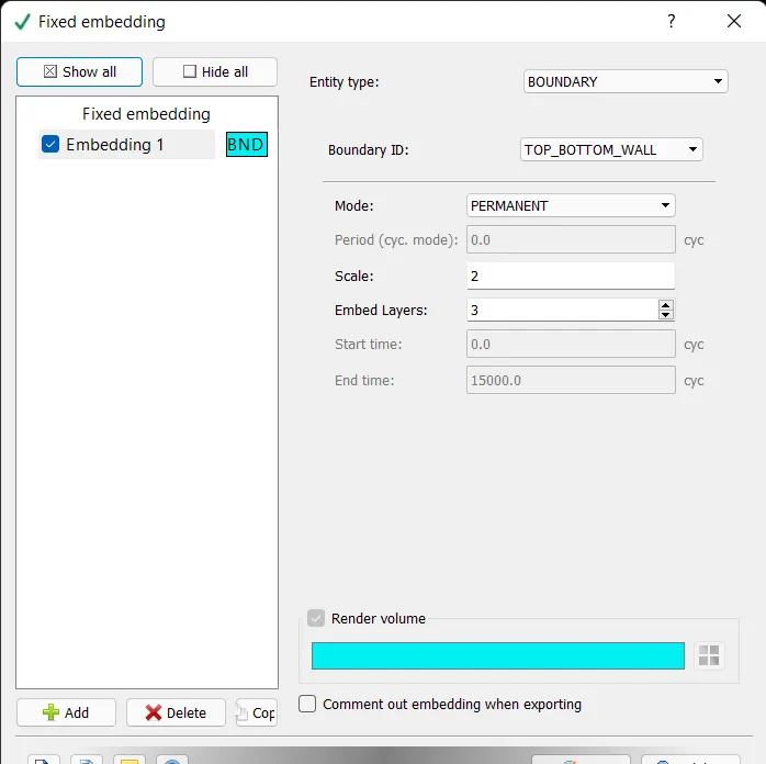
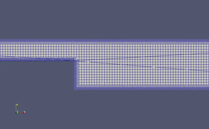
- In grid control fixed embedding is enabled and under fixed embedding scale is set to 2 and the number of layers is set to 3, then mesh size is varied for 3 cases
- Finally normals were checked an ensured that they were pointing inside of the geometry
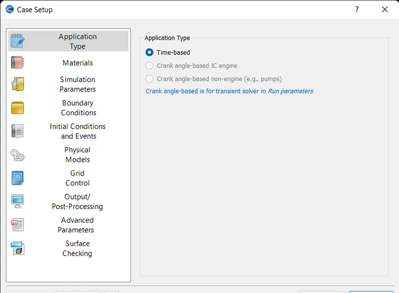
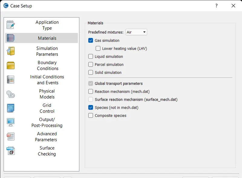
Running the simulation
- Inorder to run the simulation the input files are exported to a specified folder
- Then 'mpiexec.exe' file is copied from the convergent science directory -> converge -> 3.0.16 -> bin -> mpi -> intel64 -> bin
- Also another file named 'converge.exe' is also copied and pasted to the same folder . This file is availible in the Convergent_Science -> CONVERGE -> 3.0.16 -> bin -> msmpi folder
- CYGWIN is run as administrator and navigated to the folder containing the input files
- Then the following command is typed to start the calculation 'mpiexec.exe -n 4 converge.exe restricted' to run with 4 processors
Post processing
- After running the simulation the output files are availble in the same folder
- We can check whether the simulation has converged or not using the convergant studio line plotting, mass flow rate , velocity , pressure at inlet and outlet are obtained here
- For extracting the contour we need 3D files in output folder to be opened through paraview
- So inorder to make the files readable in paraview they are converted to either vtk file or case file. The conversion is done in Post processing in Convergant studio
- Plot over line option helps to obtain the plots of pressure drop along the pipe and the velocity variation of flow across the pipe
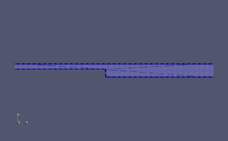
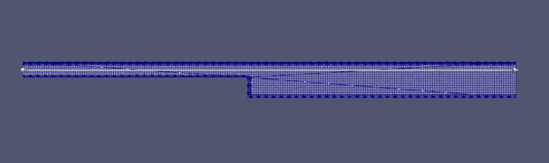
Mesh
Case-1, mesh size = 0.002
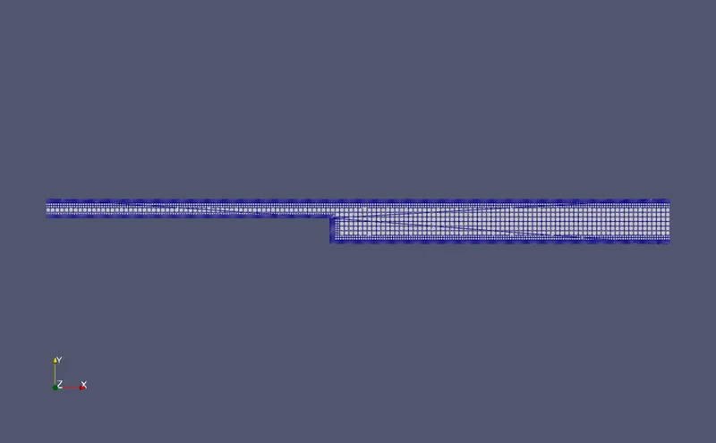
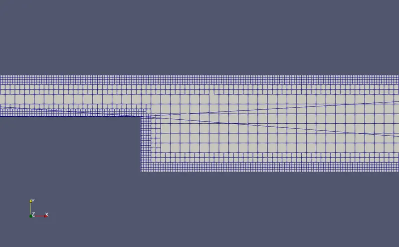
Case-2, mesh size = 0.0015
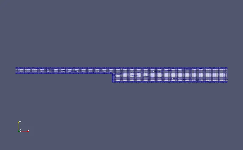
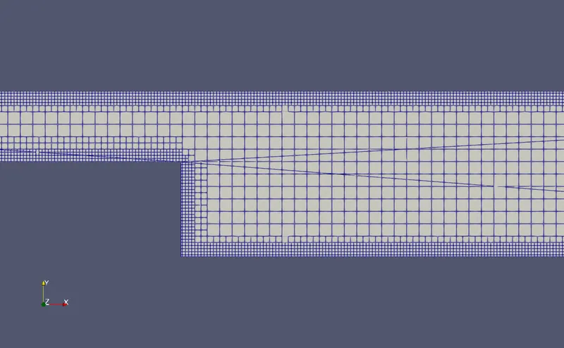
Case-3, mesh size = 0.001
Outputs
Convergancy Proof
Case-1,Mesh 0.002
Case-2,Mesh 0.0015
Case-3,Mesh 0.001
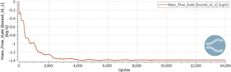
- Since we have a stable slopes obtained from above all the cases we can assure that all the solutions are converged
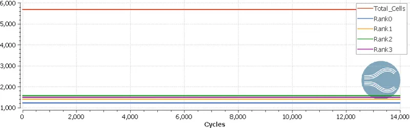
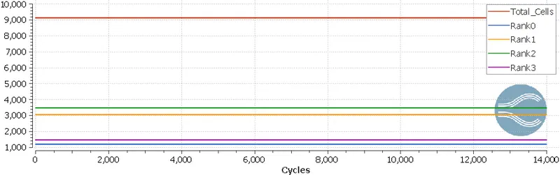
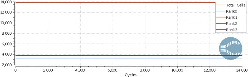
Total cell count
Case-1,Mesh 0.002
Case-2,Mesh 0.0015
Case-3,Mesh 0.001
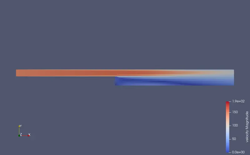
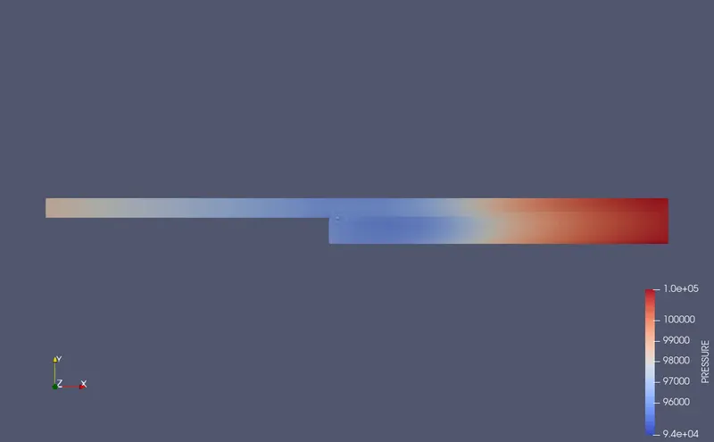
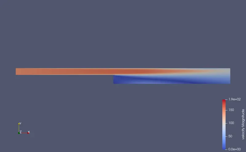
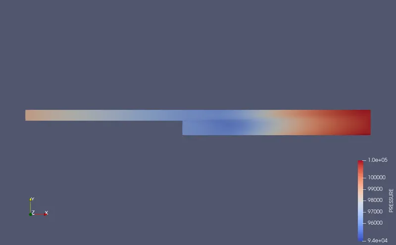
Velocity and pressure contours
Case-1,Mesh 0.002
Case-2,Mesh 0.0015
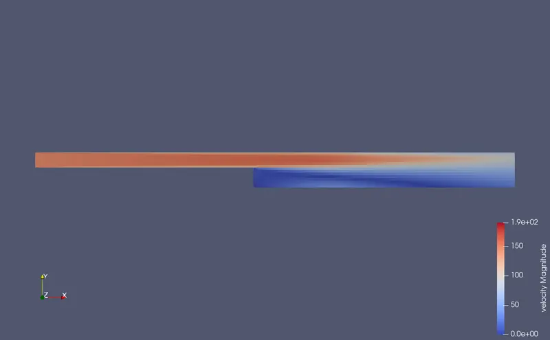
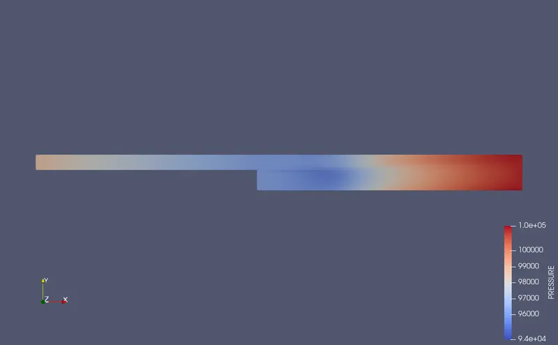
Case-3,Mesh 0.001
Plots
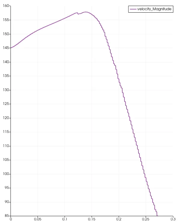
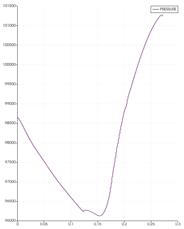
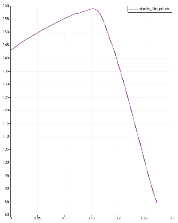
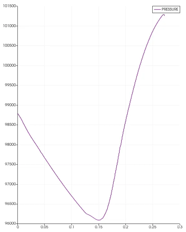
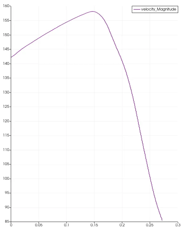
Pressure and velocity plots along the flow
Case-1,Mesh 0.002
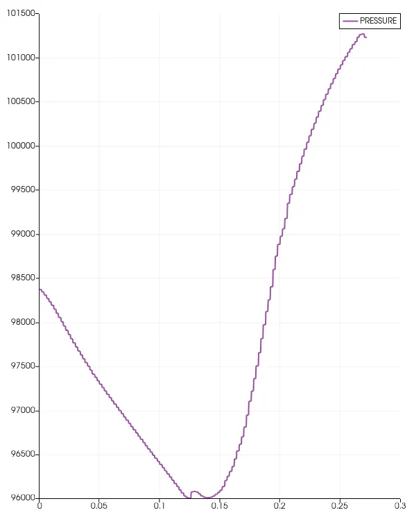
Case-2,Mesh 0.0015
Case-3,Mesh 0.001
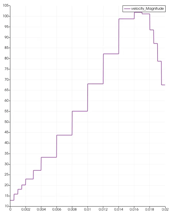
Velocity plots across the flow
Case-1,Mesh 0.002
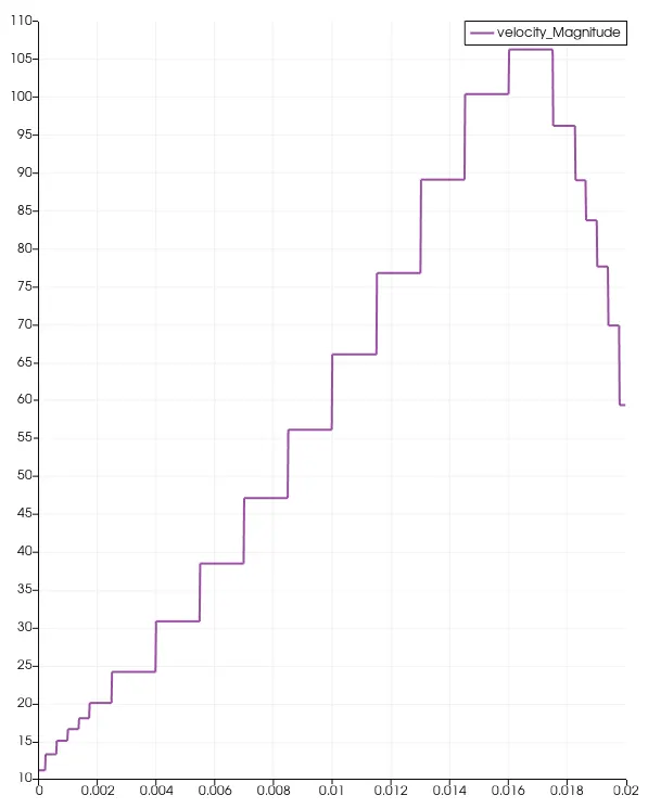
Case-2,Mesh 0.0015
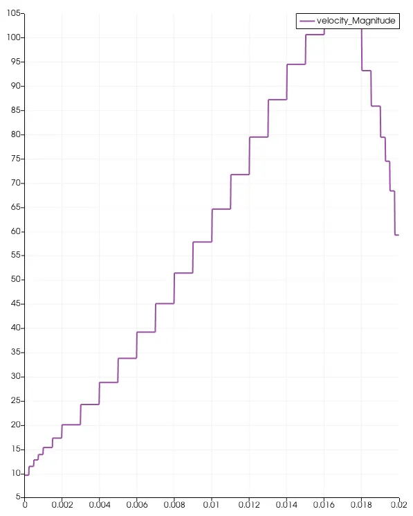
Case-3,Mesh 0.001
Results obtained
- The flow seperation occurs at the point where there is a suddent change in the geometry (step).As said earlier here the flow seperation have happened due to tha fact that the flow is no longer availible to follow the geometry due to sudden chnge in its shape. We can ensure this by taking a look at the velocity contours obtained
- We had most detailed solution is case 3
- Unlike the pressure contour of a normal 2D channel the pressure at the outlet becomes more due to change in its shape and this can lead to more disturbed fluid flow(turbulent) and also the velocity at the end is also lowered due to this phenomena
- Since we have used the RANS turbulence model the turbulence recorded here is lower
- The pressure and velocity plots along the flow implies the above explained theory
- The velocity plot across near to the outlet shows how the turbulent it has become
Conclusion
- Problem was run for three cases of mesh sizes
- Obtained the flow seperation point
- Obtained velocity and pressure contours
- Obtained relevent plots to explain the theory
- Obtained mass flow rate at the inlet to check the convergancy