Week 3: Flow over a backward facing step
FLOW OVER A BACKWARD FACING STEP
Aim:-
To simulate the flow over a Backward Facing Step with three different mesh size and shows the contour plots and line plots for three different variables.
Introduction:-
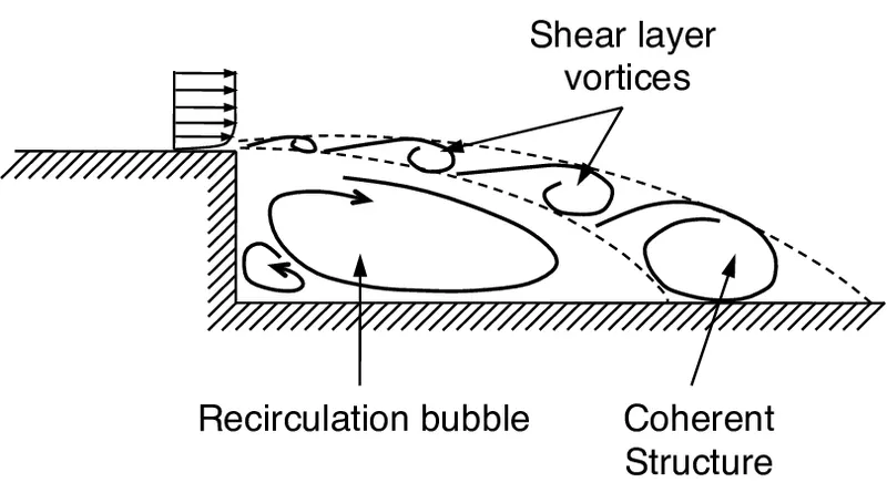
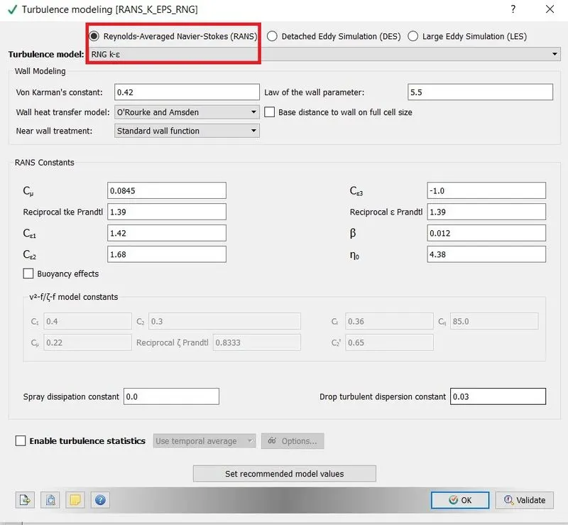
Backward Facing Step (BFS) is widely known for its application in the studies on turbulence in internal flows. The flow separation is caused due to sudden changes in the geometry. This creates a zone of re-circulation and a point of flow reattachment. Steady State RNG k-ε turbulence model was used for conducting the numerical simulation in Converge CFD.
Simulation Process
A. Geometry Setup:-
Creating geometry:-
- The vertex should be created to draw a Backward Facing Step using the "Vertex" command (Geometry Dock > Create > Vertex > Vertex by coordinate)
- The 7 vertexes is required to create a Backward Facing Step.
- Each vertex should be created by entering the coordinates value.
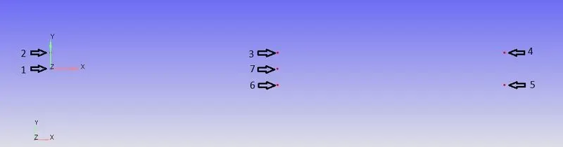
Coordinates,
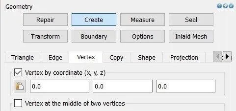
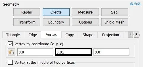
Fig(a). Vertex 1 Fig(b). Vertex 2
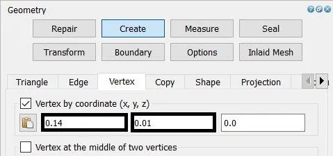
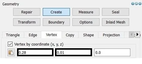
Fig(c). Vertex 3 Fig(d). Vertex 4
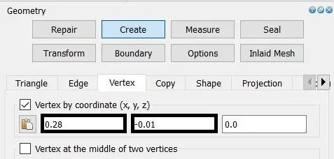
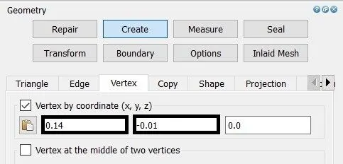
Fig(e). Vertex 5 Fig(f). Vertex 6
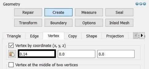
Fig(g). Vertex 7
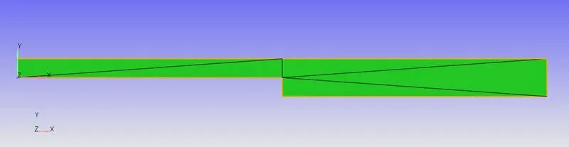
- After creating the vertex join them using the "From three vertices" command. (Geometry Dock > Create > Triangle >From three vertices)
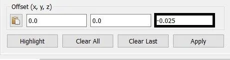
- Copy the geometry and offset it in Z-direction. (Geometry Dock > Create > Copy > Offset Distance)
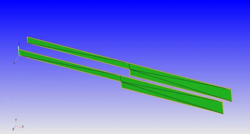
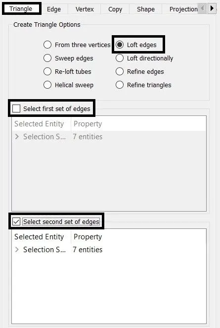
- After Offset the two set of edges has been closed using the "Loft Edge" command. (Geometry Dock > Create > Triangle > Loft Edges)
- Select the front side as the first set of edges and the back side as a second set of edges.
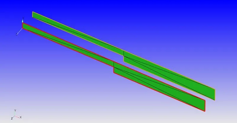
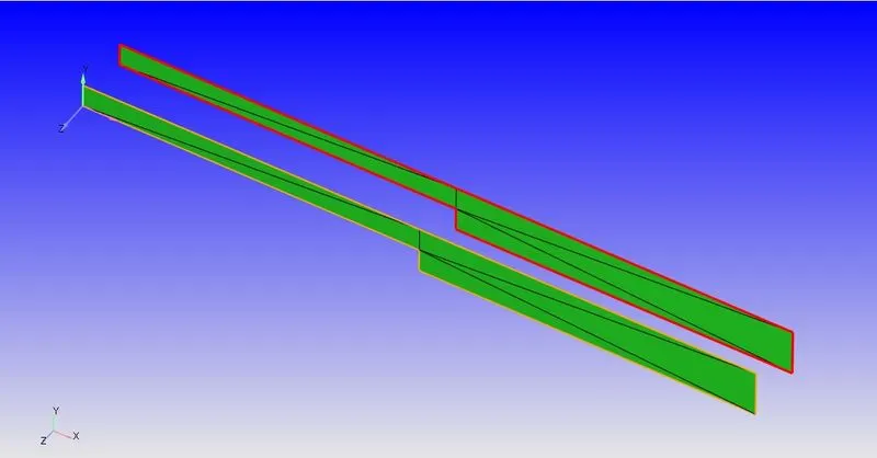
Fig(a). The First set of Edges Fig(b). The second set of Edges
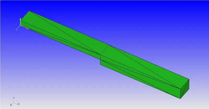
Fig(c). After creating the Loft edges
Boundary Flagging:-
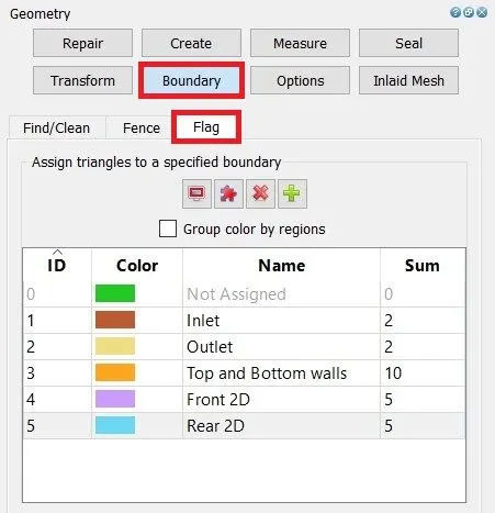
In the boundary tab, the name of the boundary and the surface has been defined under the Flag option.
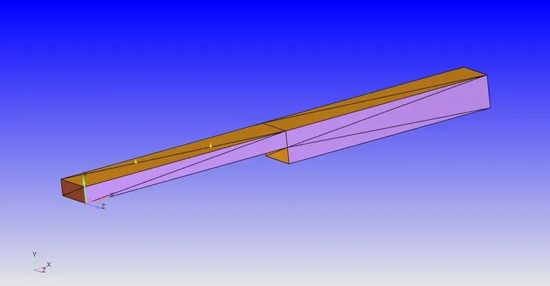
Fig(a). Boundary regions
B. Case Setup:-
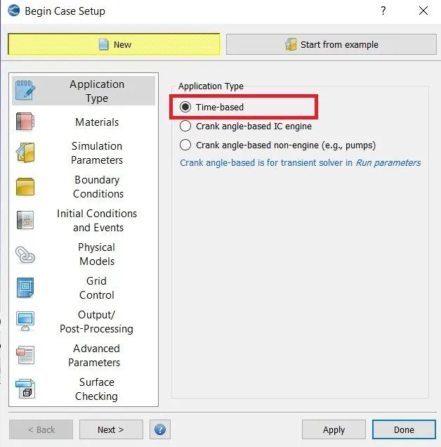
1. Application Type:-
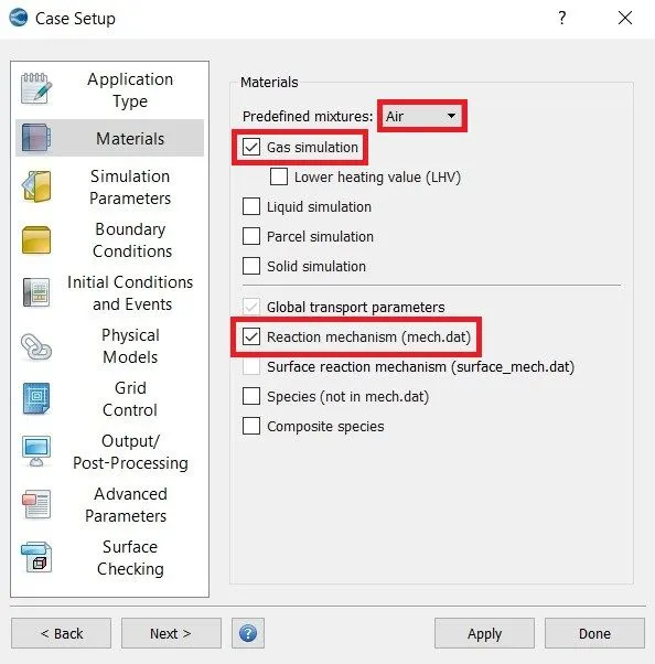
2. Material:-
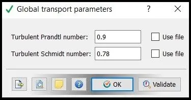
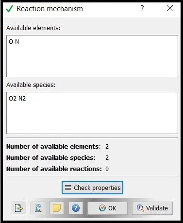
3. Simulation Parameters:-
- Steady-state solver is used.
- The steady-state monitor is enabled.
- Use share memory is unchecked.
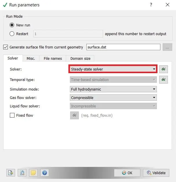
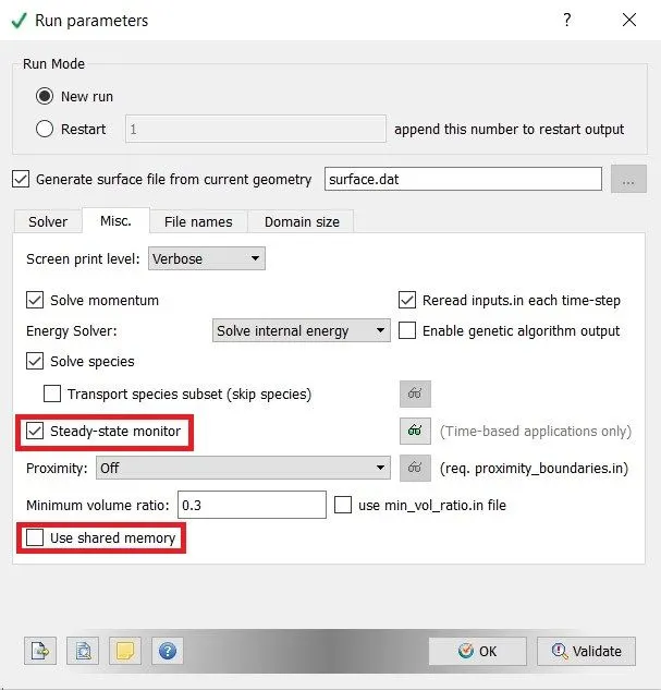
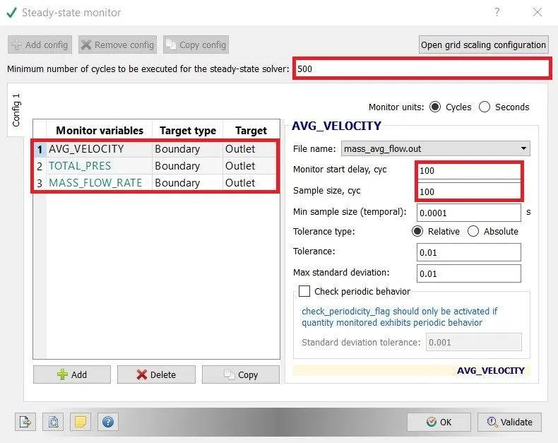
4. Steady-State monitor:-
- Average Velocity, Total Pressure and Mass flow rate is monitored.
- Minimum number of cycles to be executed for the steady-state solver is 500.
- Monitor start delay and sample size = 100 cycles.
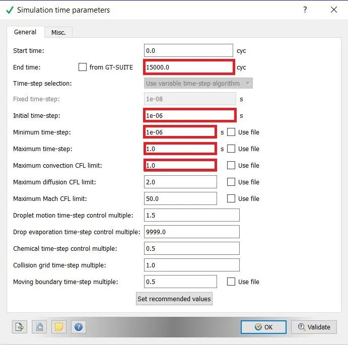
5. Simulation Time Parameters:-
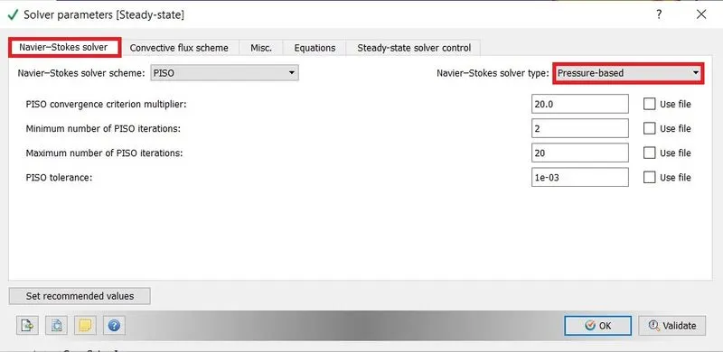
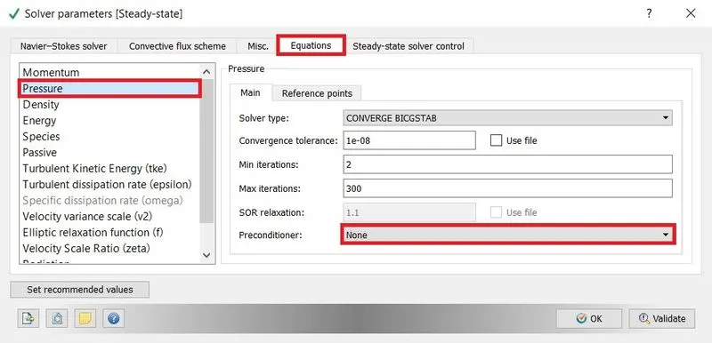
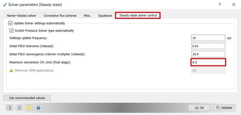
6. Solver Parameters:-
- A pressure-based solver is used.
- Maximum CFL limit for final stage is = 0.5.
- The preconditioned for pressure equation is set to be None.
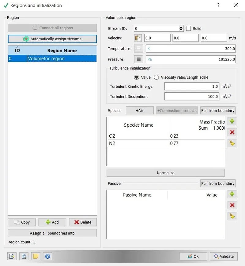
7. Region and Initialization:-
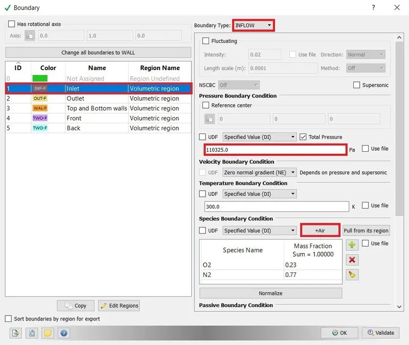
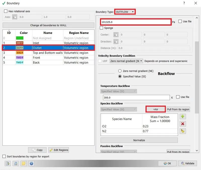
8. Boundary Conditions:-
- Inlet = Inflow with pressure 110325 Pa
- Outlet = Outflow with pressure 101325 Pa
- Top and Bottom walls = Wall with No-slip condition.
- Front 2D = Two_D
- Back 2D = Two_D
All the boundary condition is assigned with the Volumetric region.
9. Physical Model:-
10. Grid Control:-
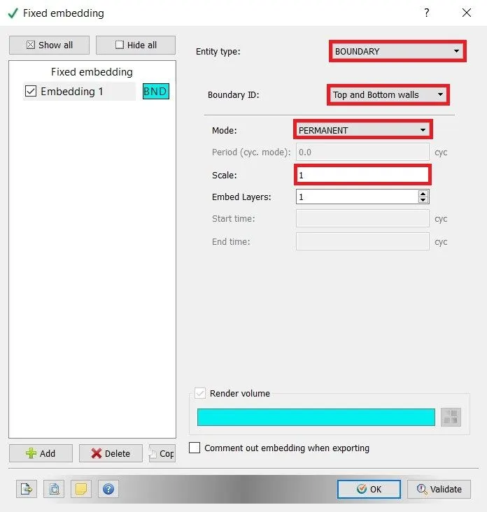
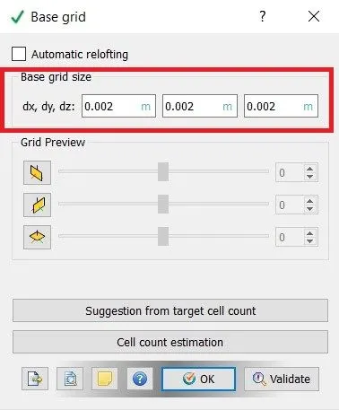
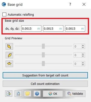
- Base grid.
- Fixed embedding.
Base mesh for 3 cases,
Case_1 = dx,dy,dz = 0.002m
Case_2 = dx,dy,dz = 0.0015m
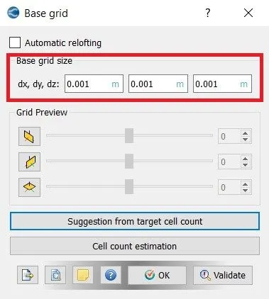
Case_3 = dx,dy,dz = 0.001m
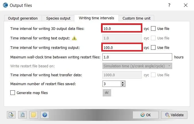
11.Output/Post-processing:-
- writing time intervals = 10 cycles
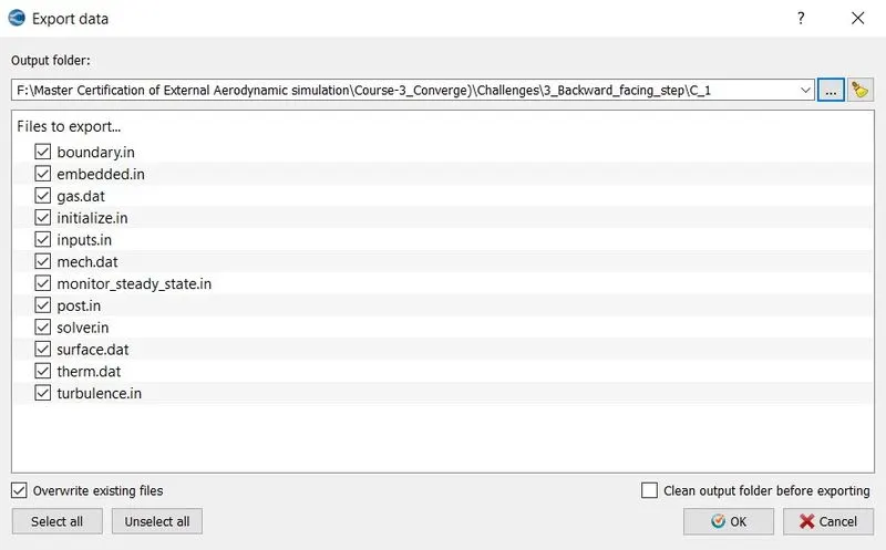
12. Export Data:-
Export all the input files to run the simulation in Cygwin.
*****************************************************************************************
Case -1 [ Base Mesh size of 0.002m]
Mesh:-

Execute the Simulation:-
- The executable mpiexec.exe and converge.exe are pasted in the input files.
- To run the simulation in Cygwin using the command.
mpiexec.exe -n 2 converge.exe restricted </dev/null> logfile &
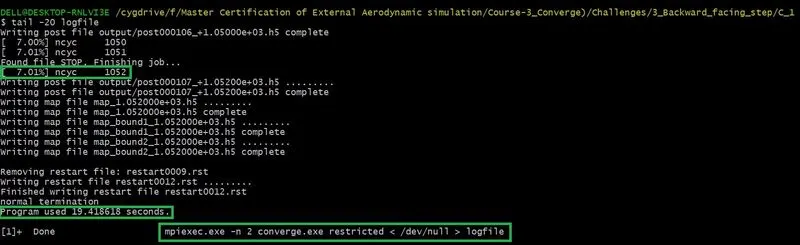
- Converge at 1052 cycles
- Time taken = 19.41 sec
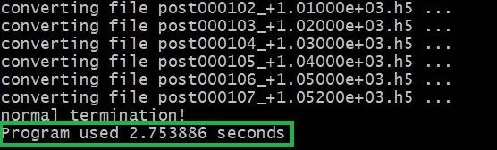
After the simulation is complete, the output files can be converted into Paraview VTK in-line binary Format to Post-process the result in Paraview.
mpiexec.exe -n 2 post_convert_30_msmpi.exe
Post-Processing Result:-
1. Contour:-
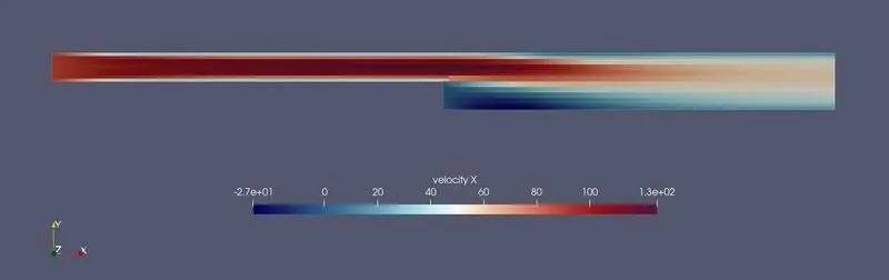
Fig(a). Velocity Contour
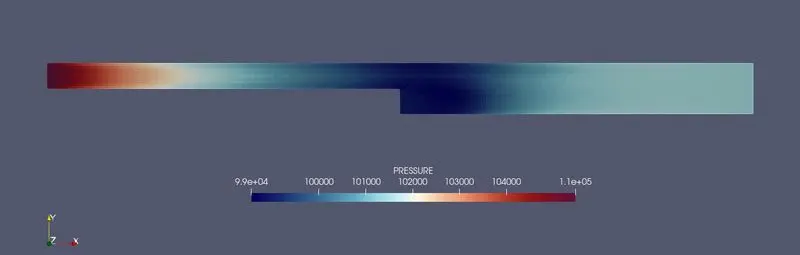
Fig(b). Pressure Contour
2. Line Plot:-
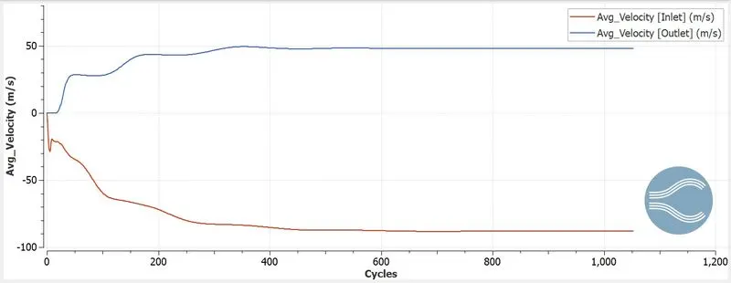
Fig(a). Average Velocity
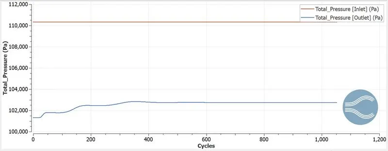
Fig(b). Total Pressure
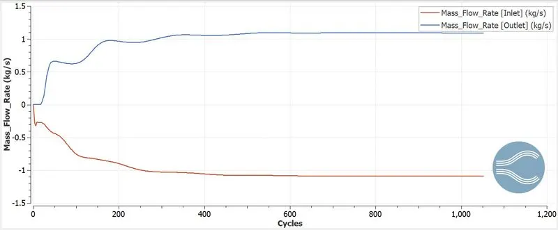
Fig(c). Mass Flow Rate
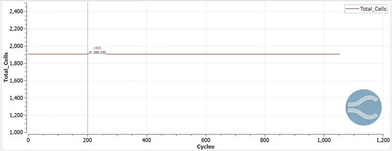
Fig(d). Total Cell
Total cells count = 1905
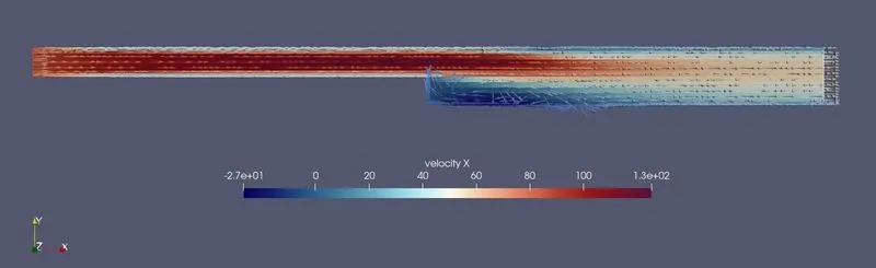
3. Flow separation:-
4. Animation:-
*****************************************************************************************
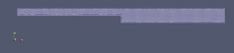
Case -2 [ Base Mesh size of 0.0015m]
Mesh:-
Execute the Simulation:-
- The executable mpiexec.exe and converge.exe are pasted in the input files.
- To run the simulation in Cygwin using the command.
mpiexec.exe -n 2 converge.exe restricted </dev/null> logfile &
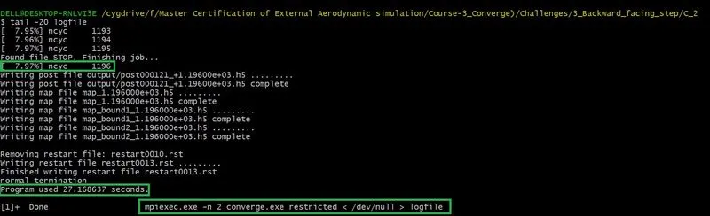
- Converge at 1196 cycles
- Time taken = 27.17 sec
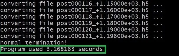
After the simulation is complete, the output files can be converted into Paraview VTK in-line binary Format to Post-process the result in Paraview.
mpiexec.exe -n 2 post_convert_30_msmpi.exe
Post-Processing Result:-
1. Contour:-
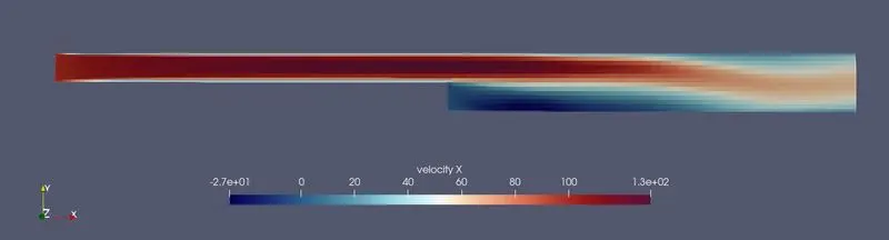
Fig(a). Velocity Contour
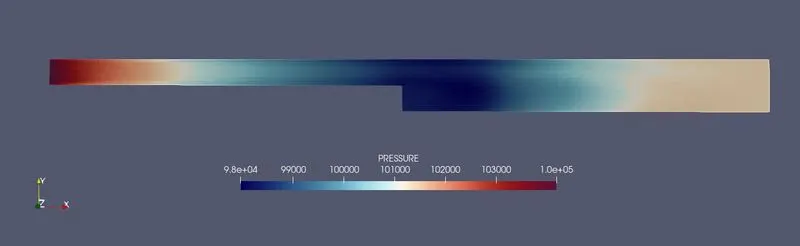
Fig(b). Pressure Contour
2. Line Plot:-
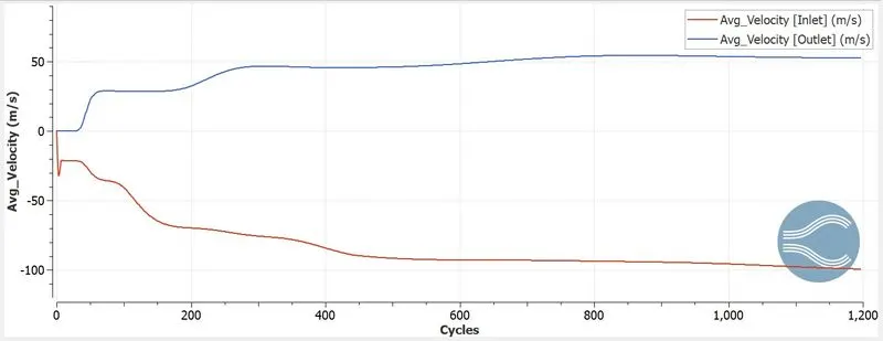
Fig(a). Average Velocity
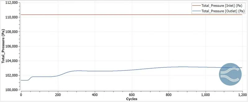
Fig(b). Total Pressure
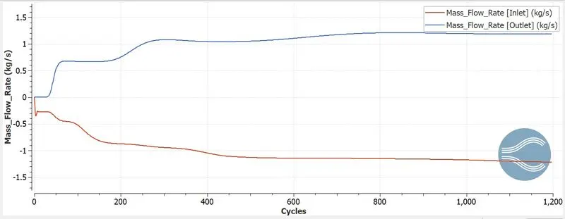
Fig(c). Mass Flow Rate
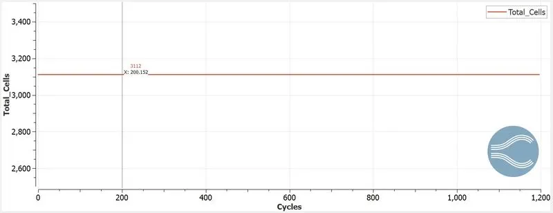
Fig(d). Total Cell
Total cells count = 3112
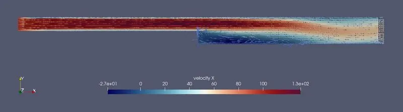
3. Flow separation:-
4. Animation:-
*****************************************************************************************
Case - 3 [ Base Mesh size of 0.001m]
Mesh:-

Execute the Simulation:-
- The executable mpiexec.exe and converge.exe are pasted in the input files.
- To run the simulation in Cygwin using the command.
mpiexec.exe -n 2 converge.exe restricted </dev/null> logfile &
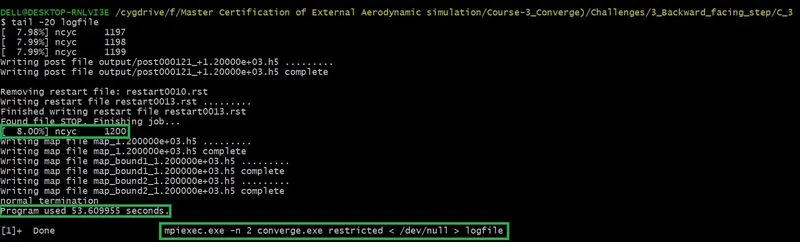
- Converge at 1200 cycles
- Time taken = 53.60 sec
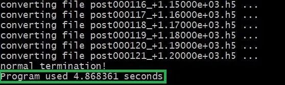
After the simulation is complete, the output files can be converted into Paraview VTK in-line binary Format to Post-process the result in Paraview.
mpiexec.exe -n 2 post_convert_30_msmpi.exe
Post-Processing Result:-
1. Contour:-
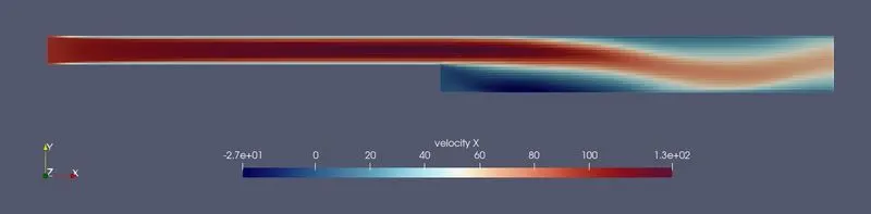
Fig(a). Velocity Contour
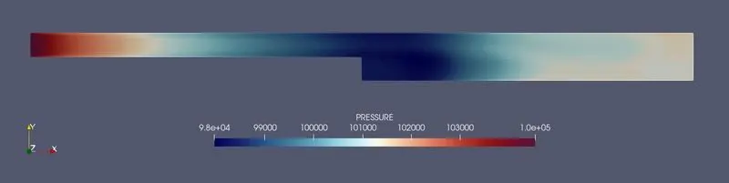
Fig(b). Pressure Contour
2. Line Plot:-
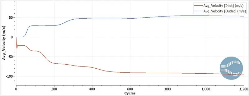
Fig(a). Average Velocity
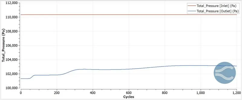
Fig(b). Total Pressure
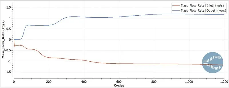
Fig(c). Mass Flow Rate
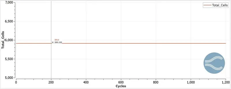
Fig(d). Total Cell
Total cells count = 5910
3. Flow separation:-
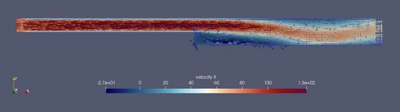
4. Animation:-
Where and why Separation is taking place.
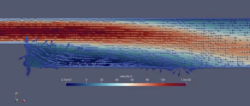
The flow separation is taking place in the region behind the step and the flow is recirculated in that region. This can occur due to the sudden changes in the geometry. Due to the flow separation, the pressure is reduced in that region.
Conclusion:-
| Simulation time | No of Cycles to converge | No of Cells | |
| Case 1 | 19.41 | 1052 | 1905 |
| Case 2 | 27.17 | 1196 | 3112 |
| Case 3 | 53.60 | 1200 | 5910 |
- The simulation time and no of cells are increased when the grid size is reduced.
- The refined mesh (0.001m) shows the flow of velocity clearly in velocity contour.
- The velocity and pressure are decreased in the recirculation region.
- From the Pressure plot, inlet pressure is constant in all cases.
- The velocity plot shows, the inlet velocity is about 100m/s and the outlet nearly about to 50m/s. So, the velocity is reduced at the outlet.
- The mass flow rate at the outlet is nearly about 1kg/s.
- There is no change in the total cell count in all the cases. so, there is no loses in cell count in the simulation.
- From the simulation, the flow can be separated due to sudden changes in the geometry and creates the recirculation zone.
Animation Link:-
Case 1 - Backward Facing Step with a Mesh size of 0.002m