Week 3: Flow over a backward facing step

FLOW OVER A BACKWARD FACING STEP

AIM: To simulate the flow over a backward-facing step with three different case base mesh sizes.

OBJECTIVE:

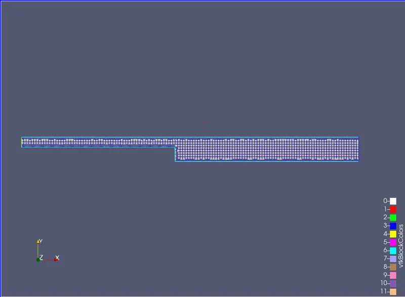
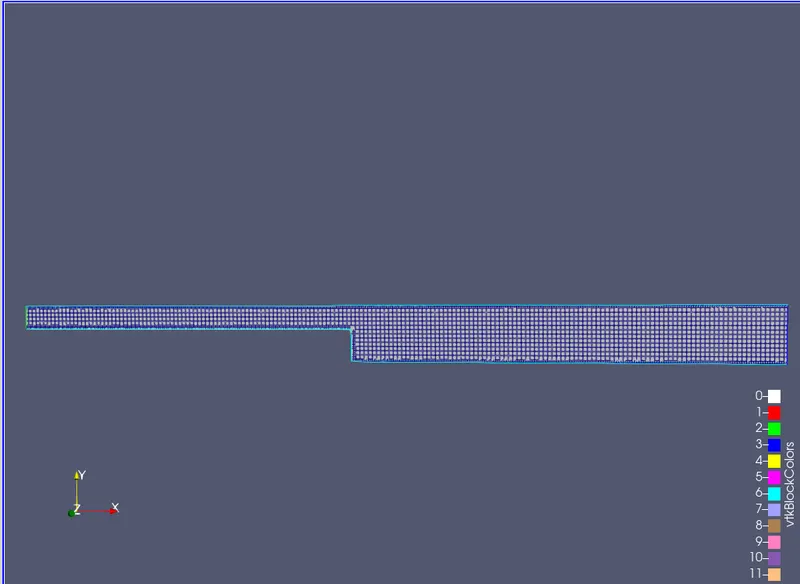
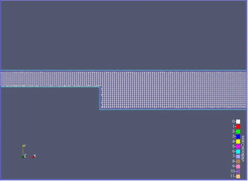
1. Show the mesh (i.e surface with edges) for all the 3 base mesh sizes

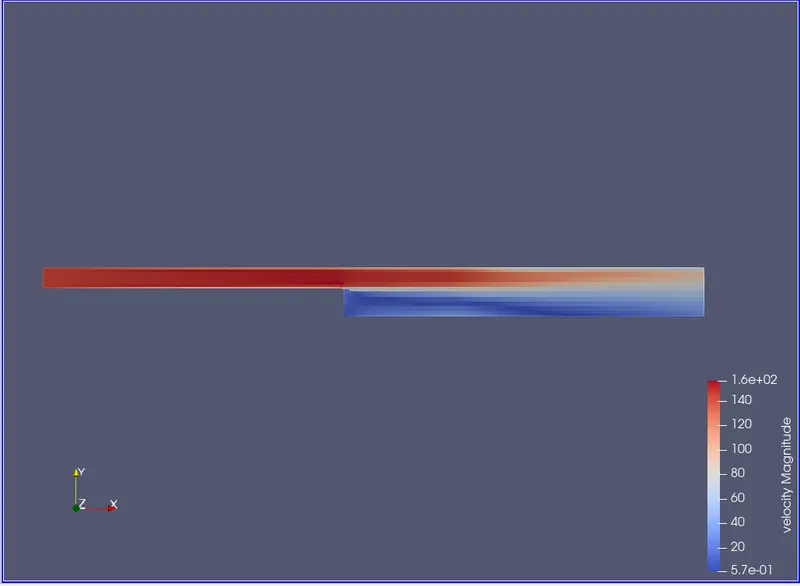
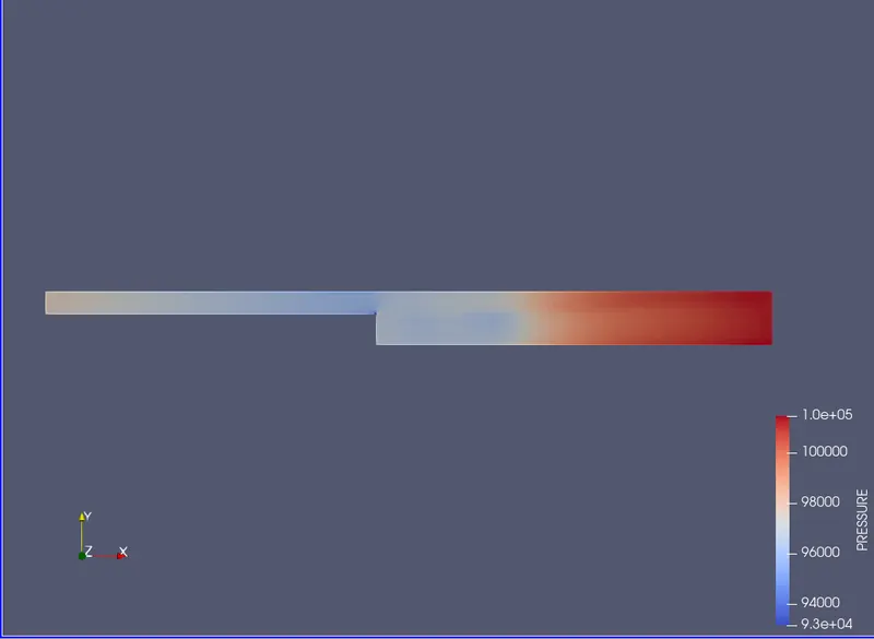
2.Show pressure and velocity contours

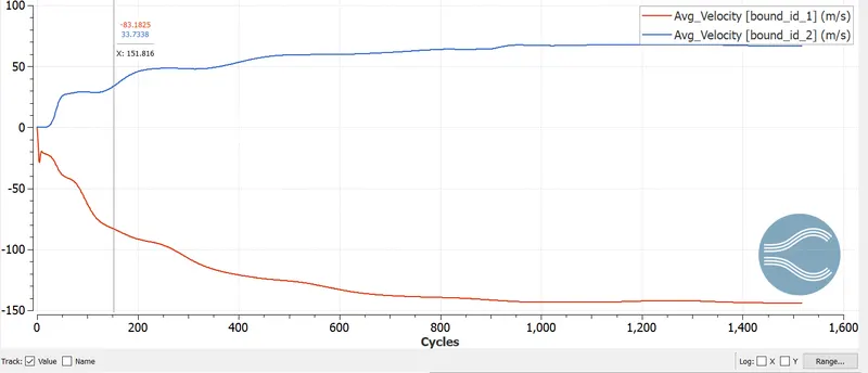
3. Show the plots of velocity, pressure, mass flow rate, and total cell count for all the 3 base mesh sizes

4. Also explain where and why separation is taking place in detail.

Make sure you make your project public. Once you are done, paste the link to your project here.

THEORY:

Backward-Facing Step (BFS) flow is one representative model for separation flows, which can be widely seen in aerodynamic flows (airfoil, spoiler, high attack angle process), engine flows, condensers, vehicles (cars, boat), heat transfer systems, and even the flow around buildings, etc. The flow separation after a simple stage will introduce separation bubble formation, evolution, and re-attachment process, which is dependent on the BFS geometric design, the inlet and outlet conditions, turbulent intensity, as well as heat transfer conditions. In the past decades, it has been widely studied by various theoretical, experimental, and numerical methods.

SETUP AND SOLUTIONS:

In this project, we run 3 different cases based on the mesh. They are:

Case1 :dx = dy = dz =2e-3 m

dx = dy = dz =1.5e-3 m

Case3: dx = dy = dz =1.0e-3 m

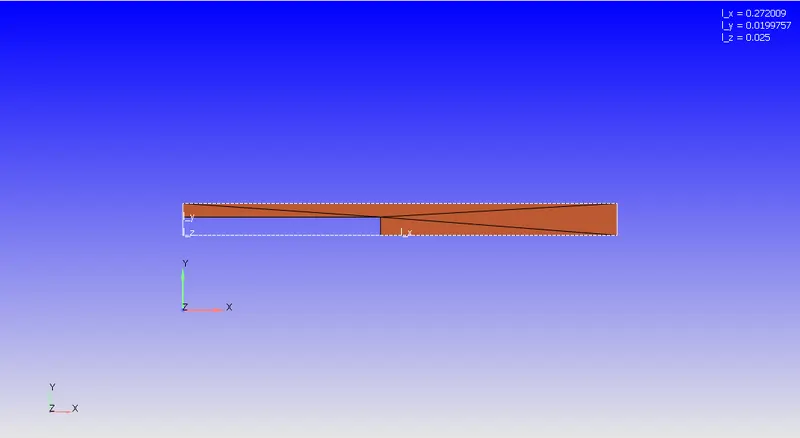
Geometry:

With the given dimension we create the geometry using the vertices and using sweep edges and extending the geometry.

Setup:

SETUP
Application Type	Time-based
MATERIALS:
1. Gas simulation	Standard
2. Global Transport Parameters	Standard
3. Reaction Mechanism	Standard
SOLUTION PARAMETERS
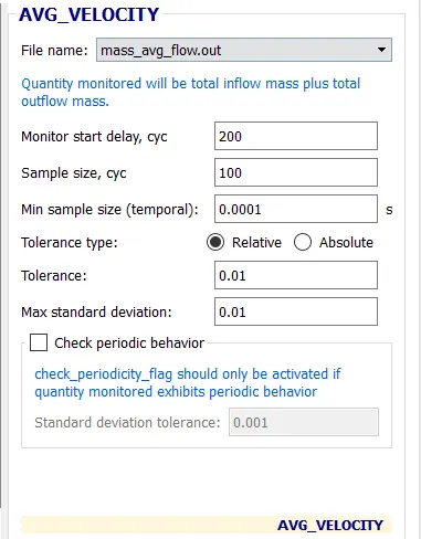
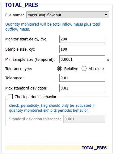
1. Run Parameters Steady-state monitor:	Steady-state solver>Full hydrodynamic>Compressible AVG_Velocity TOTAL_Pressure
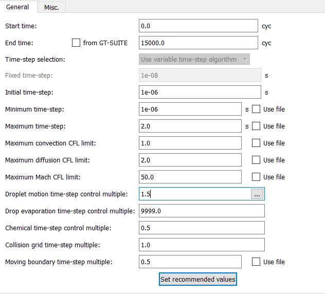
2. Simulation time parameters
3. Solver parameters	Navis-stokes solver scheme: PICO Navis-stokes solver type: pressure-based Max convection CFL limit: 0.5
BOUNDARY CONDITIONS
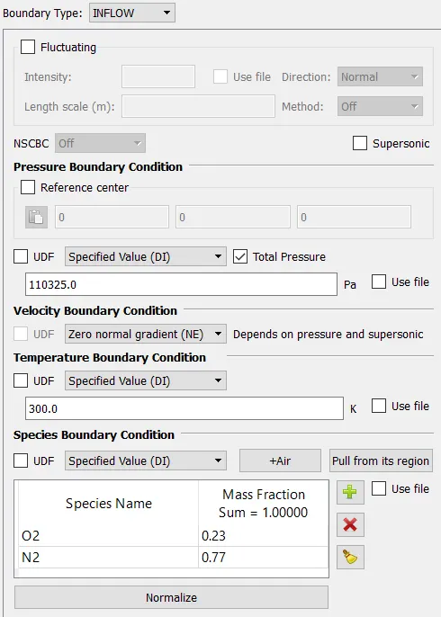
1. Inlet
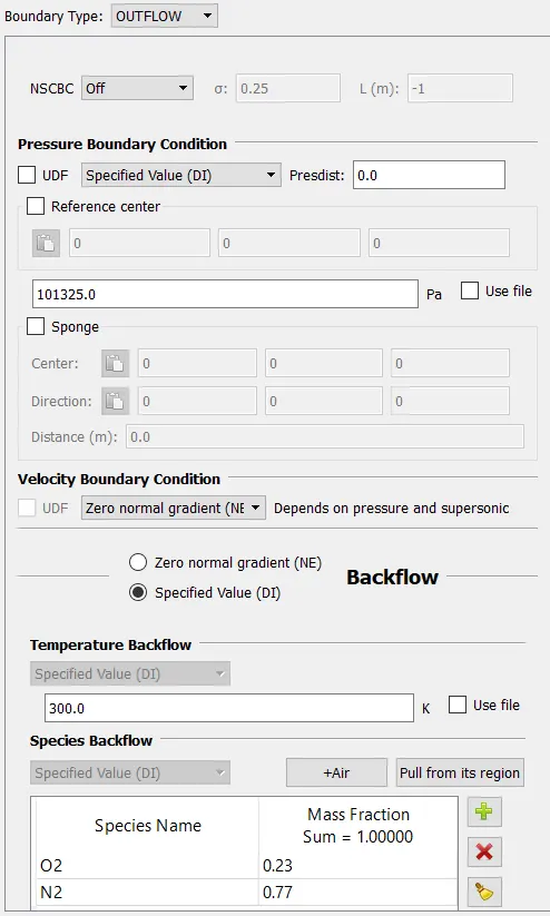
2. Outlet
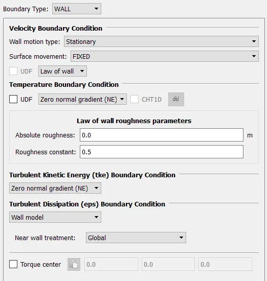
3. Top and bottom wall
4. Front wall	2-D Wall
5. Back wall	2-D wall
INITIAL CONDITIONS AND EVENTS
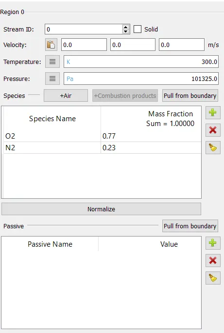
1. Regions and initialization
PHYSICAL MODELS	RNG- k-epsilon
GRID CONTROL
1. Base mesh	3 cases Case 1: dx = 2e-3m, dy = 2e-3m and dz = 2e-3m Case 2: dx = 1.5e-4m, dy = 1.5e-4m and dz = 1.5e-4m Case 3: dx = 1.0e-3m, dy = 1.0e-3m and dz = 1.0e-3m
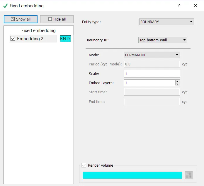
2. Fixed embedding
OUTPUT/POST-PROCESSING
1. Post variable selection	Standard
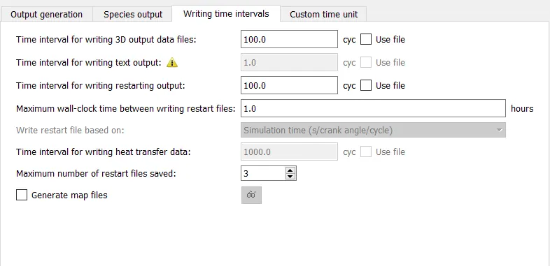
2. Output files:

Then Export the Files

Then continuing the setup in Cygwin :

• leading to the folder where the exported files are saved
• Then using mpiexec.exe -n 2 converge.exe restricted to simulate the setup
• After the output is generated, we lead the Cygwin to the output folder, and by copying the post_convert folder and
• Using mpiexec.exe -n 2 post_convert.exe and converting these files for processable output in ParaView.

Meshing

Case 1: dx = 2e-3m, dy = 2e-3m and dz = 2e-3m

Case 2: dx = 1.5e-4m, dy = 1.5e-4m and dz = 1.5e-4m

Case 3: dx = 1.0e-3m, dy = 1.0e-3m and dz = 1.0e-3m

Solution

Case 1: dx = 2e-3m, dy = 2e-3m and dz = 2e-3m

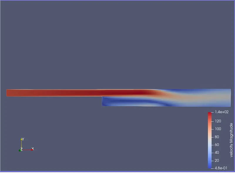
VELOCITY COUNTER

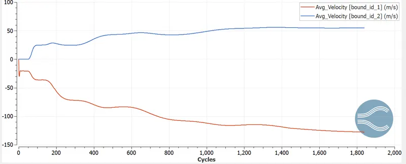
VELOCITY PLOT

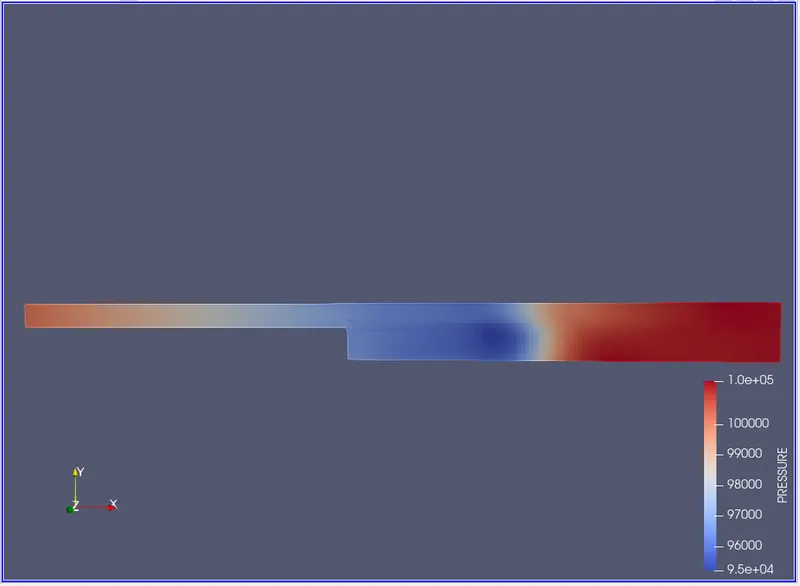
PRESSURE COUNTER

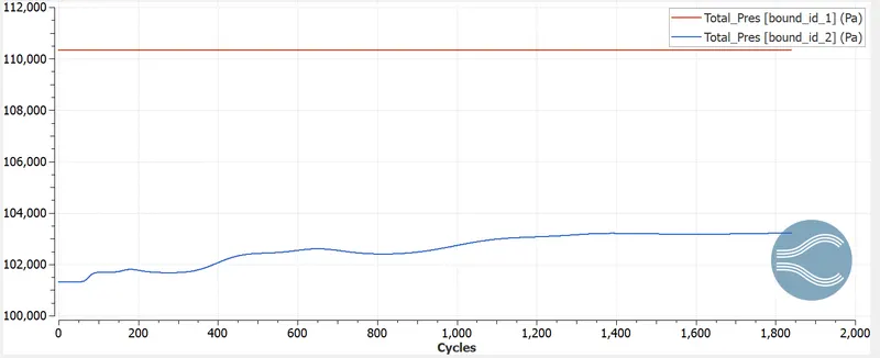
PRESSURE PLOT

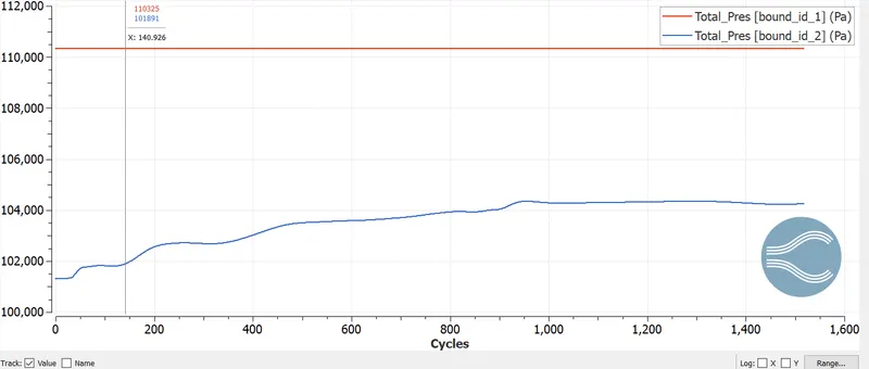
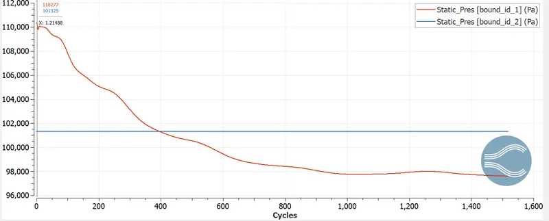
MASS FLOW RATE

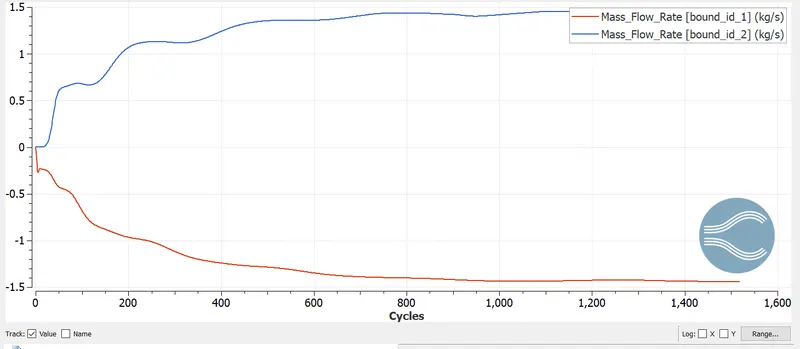
CELL COUNT

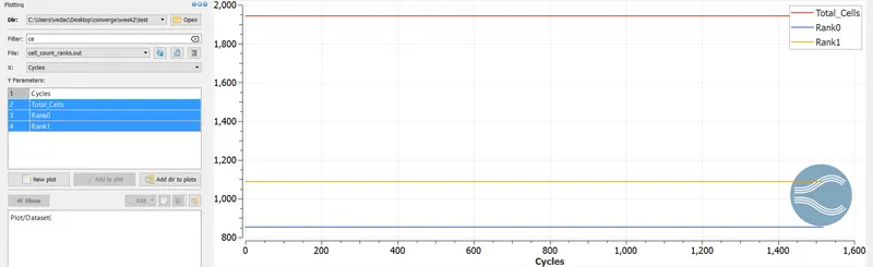
ANIMATION

VELOCITY:https://youtu.be/xwToB2lrNxo

PRESSURE:https://youtu.be/Pp7GP-542Qc

Case 2: dx = 1.5e-4m, dy = 1.5e-4m and dz = 1.5e-4m

VELOCITY COUNTER

VELOCITY PLOT

PRESSURE COUNTER

PRESSURE PLOT

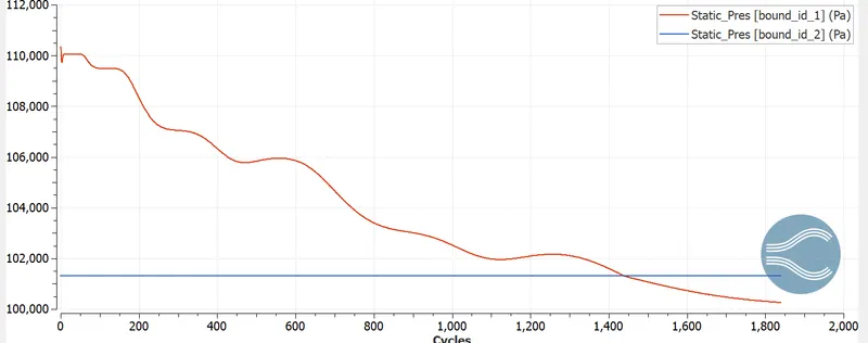
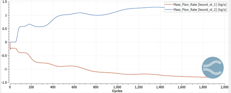
MASS FLOW RATE

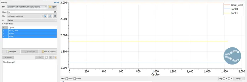
CELL COUNT

ANIMATION

VELOCITY:https://youtu.be/DmchxebfvZA

PRESSURE:https://youtu.be/l3-MJrgETC0

Case 3: dx = 1.0e-3m, dy = 1.0e-3m and dz = 1.0e-3m

VELOCITY COUNTER

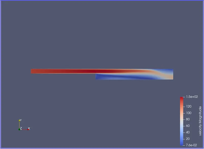
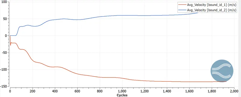
VELOCITY PLOT

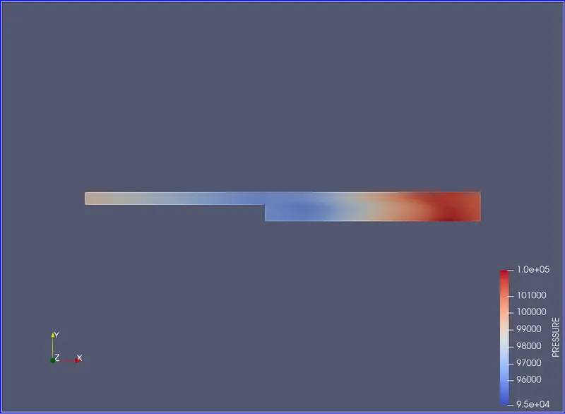
PRESSURE COUNTER

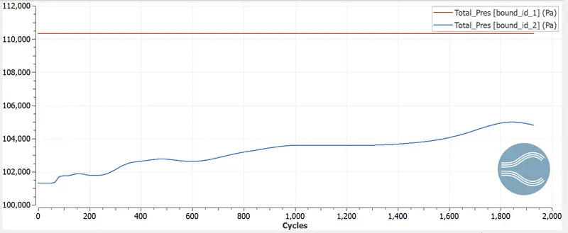
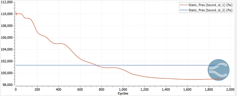
PRESSURE PLOT

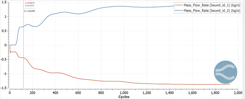
MASS FLOW RATE

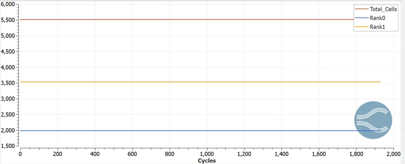
CELL COUNT

ANIMATION

VELOCITY:https://youtu.be/g64bs3PqUio

PRESSURE:https://youtu.be/kbp4heEIMUs

CONCLUSIONS

1. As we decrease the grid size, the cells count and computational time increases.
2. Damping of the disturbances depends on the base grid size, the smaller the base grid size more cycles are taken to damp completely and achieve a steady state. Whereas in our case, we are able to achieve a steady state for each of them
3. Vortices are formed at the region of flow separation.
4. Static pressure decreases in the recirculation region.
5. As the grid size reduces, more accurate point of flow separation can be seen
6. The total pressure drops at the outlet inferred the flow direction from the inlet to outlet.
7. At the outlet, the velocity was lower in comparison to inlet velocity due to BFS.
8. For all three cases, the mass flow rate is conserved through the backward-facing step channel flow.