Week 3: Flow over a backward facing step
Aim: Flow over a backward-facing step
Objective: The simulation is run for the three different mesh size
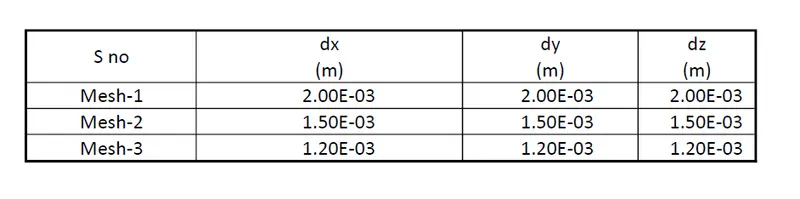
Contents to be shown in the report:
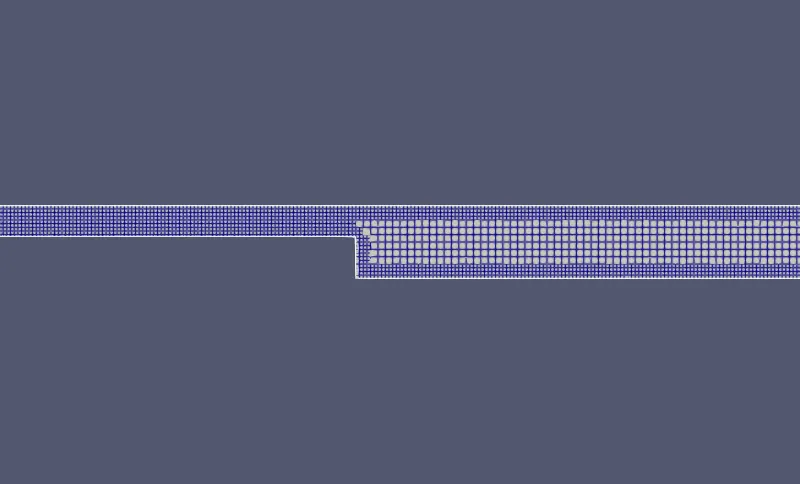
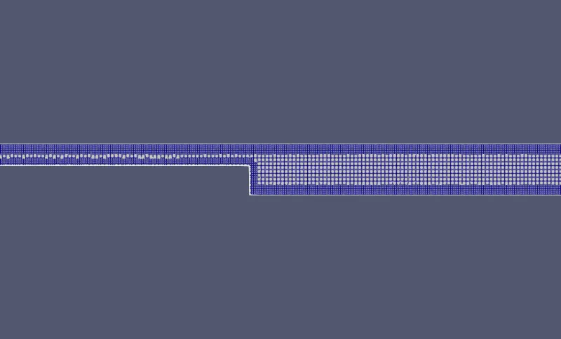
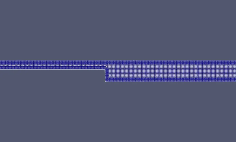
1. Show the mesh (i.e surface with edges) for all the 3 base mesh sizes
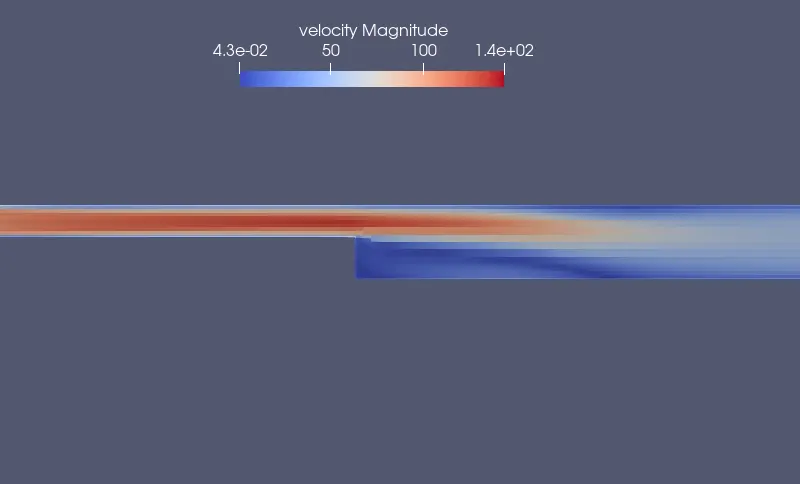
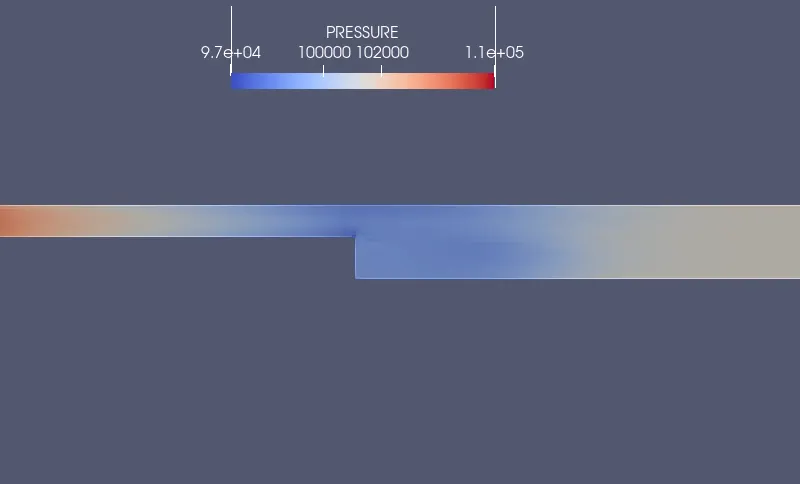
2. Show pressure and velocity contours
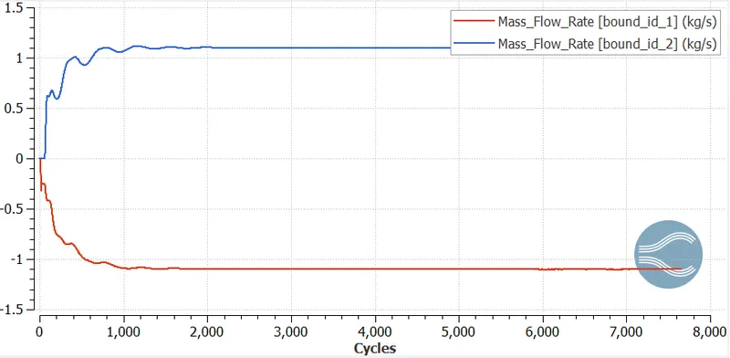
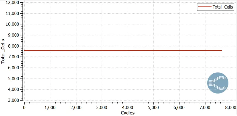
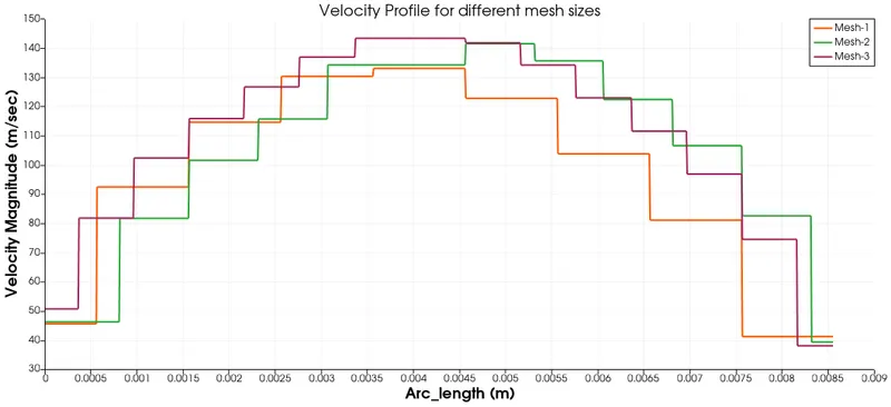
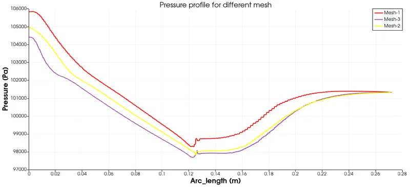
3. Show the plots of velocity, pressure, mass flow rate, and total cell count for all the 3 base mesh sizes
4. Also explain where and why separation is taking place in detail.
Introduction
Backward-facing
The backward-facing step is widely used for its application of turbulence in internal flows. The flow separation is caused due to the sudden changes in the geometry and the inlet and outlet pressure values. The flow separation causes a point of reattachment and a point of recirculation.
The backward-facing step represents separation flows, which can be widely seen in aerodynamic flows, heat transfer, engine flows, condensers, vehicles, and flow around the building.
Case setup
The bfs. STL file is loaded into the Converge-CFD set-up.
The "Normal Toggle" is selected from the ribbon, upon selecting the normal toggle it was observed that the normal is pointing outside the volume, technically the normal should point inside the volume where the fluid is flowing. Therefore in the geometry dock, the "Transform" option is clicked. The "Normal" tab is selected from the geometry dock and one of the triangles containing the normal pointing outward is selected. The "Apply" option is selected for removing the normals.
The diagnosis dock is selected from the "View" option and the "Find" option is selected. It is found that there is no problem observed in the geometry ("Intersections(0)","Nonmanifold Problems(0)","Open Edges(0)", "Overlapping Tris(0)","Normal Orientation(0)","Isolated tris (0)".
The "Case Setup Dock" is selected from the "View" and "Begin Case Setup" is executed.
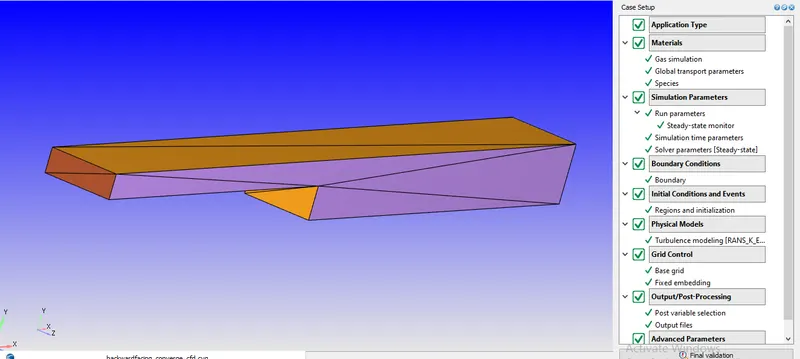
The "Time" based "Application" type is selected. The "Material" is selected and the predefined mixture is selected as air. The "Reactant mechanism" is checked off because it is not a combustion problem. The species is selected and the "Apply" is clicked. Under "Gas simulation" the Equation of state is selected as "Redlich Kwong", the critical temperature is 133K and the critical pressure is 3770000Pa. The Turbulent Prandtl number is 0.9 and the Turbulent Schmidt number is 0.78 under Global Transport parameters. The O2O2 and the N2N2 are selected as species. Under "Run parameters" the "Steady-state solver" is selected. The "Temporal type" is locked for the steady state. The "simulation mode" is selected as "Full Hydrodynamic" because the geometry is simple so while creating the mesh inside the geometry it solves the NS equation as well, but if the geometry is complex "No hydrodynamic solver" is selected as such if there is an error it will point out immediately while creating the mesh, otherwise if the hydrodynamic solver is selected then it will be very tedious to identify the error in the simulation case set up.
Under "Simulation time parameters" the end time is chosen as 15000 cycles (steady-state). The initial and minimum time step is 1e-09 s. The maximum time step is 2s, the maximum convection CFL limit is 1 and the rest are default values.
The "Pressure" "Equation" is selected under the "Solver parameter" and the "Preconditioner" is selected to "None". The "Maximum convection CFL limit (final stage)" is set to 0.5.
Boundary conditions
The boundary conditions for the different named selections are tabulated below
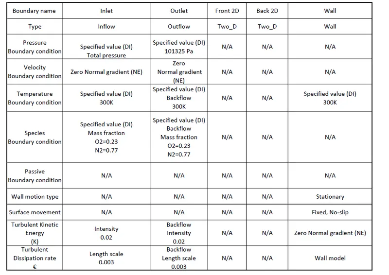
In the "Region and Initialization" the mass fraction of O2O2 and N2N2 were created and named "Region 0" and the same is updated in the boundary condition region name. These are the initial condition and will be washed out after the solution has converged.
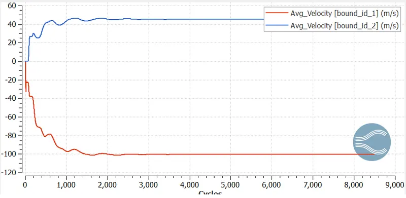
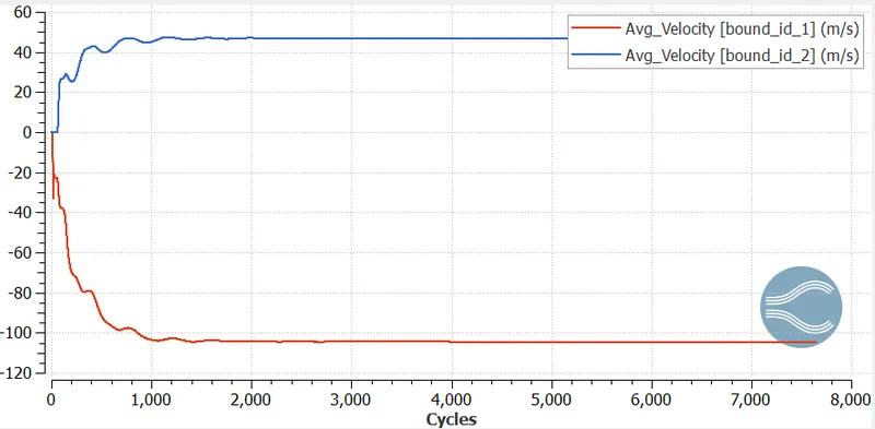
The monitor variables are added in the "Steady-state monitor". Avg Velocity, Mass flow rate has been added and the target area is selected as output. The minimum number of cycles to be executed for the steady-state solver is 5000 which signifies that the solver will run for a minimum of 5000 cycles if the solution reaches a convergence value before 5000, then the simulation will stop at 5000, but if the solution reaches a convergence value after 5000 then it will terminate at that moment. The solver checks the difference in the value of two consecutive sample sizes (1000) and matches it with the tolerance value to stop the solution. The converge-CFD software saves a lot of time and computational energy by tracking the solution when it reaches a steady state.
Setting up of Turbulence model
The Realisable k−εk-ε model is selected from the case-setup tree for the above-said simulation. Since the size of the eddies is restricted near the wall and the maximum size of the eddies is formed away from the wall. It is well-suitable for resolving flows in the logarithmic flow region where y+ ranges from 30 to 300, and for flows involving a high Reynolds number.
Determination of flow velocity
First of all, let us assume that the flow is incompressible, the Bernoulli Equation for the incompressible flow states that the sum of the mechanical, potential, and kinetic energy remains constant, so any increase in one form may result in the decrease in another form. Therefore for the above surface, the equation can be written as
Ps+12ρv2+ρgh=PtotalPs+12ρv2+ρgh=Ptotal
For the backward-facing, ρghρgh can be neglected
Therefore the equation becomes
At the inlet
Equation 1
Ps1+12ρv21=PtotalPs1+12ρv12=Ptotal
Therefore the static pressure equates to
Equation 2
Ps1=Ptotal−12ρv21Ps1=Ptotal-12ρv12
The terms in the equation have their usual meaning
Ps1Ps1 is the static pressure at the inlet
ρρ is the density of air
v1v1 is the velocity at the inlet boundary condition`
P total is the total pressure, in this case, the pressure at the inlet boundary condition.
The outlet boundary condition uses static pressure to solve the backward-facing simulation.
At the outlet
Equation 3
Ps2+12ρv22=PtotalPs2+12ρv22=Ptotal
Ps2Ps2 is the static pressure at the outlet`
ρρ is the density of air
v2v2 is the velocity at the outlet boundary condition`
Therefore PtotalPtotal can be written for the inlet and used in the above equation
Equation 4
Ps2+12ρv22=Ps1+12ρv21Ps2+12ρv22=Ps1+12ρv12
But the static pressure at the inlet is unknown, therefore using the value of Ps1Ps1 from Equation 2 and using it in Equation 4.
The new equation becomes
Equation 5
Ps2+12ρv22=Ptotal−12ρv21+12ρv21Ps2+12ρv22=Ptotal-12ρv12+12ρv12
Applying the continuity equation to get the values of v1&v2v1&v2
Equation 6
A1v1=A2v2A1v1=A2v2
A1A1 is the inlet area =H∗W=H∗W
Height of the inlet = 0.008548m0.008548m
Width of the inlet = 0.025m0.025m
Therefore A1A1=0.0002137m20.0002137m2
A2A2 is the outlet area =H∗W=H∗W
Height of the outlet=0.0199m0.0199m
Width of the outlet= 0.025m0.025m
Therefore A2A2=0.0004975m20.0004975m2
Therefore v1v2=A2A1v1v2=A2A1
v1v2=2.328v1v2=2.328
In Equation 5
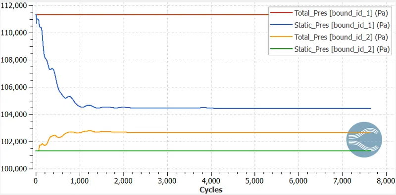
Ps2=101325PaPs2=101325Pa
Ptotal=111325PaPtotal=111325Pa
ρρ at 300K and 1atm pressure =1.177kgm3=1.177kgm3
Therefore Equation 5 becomes
v22=200001.177v22=200001.177
v2=130.354msec−1v2=130.354msec-1
v1=303.465msec−1v1=303.465msec-1
Calculating the Mach number for the flow
The Mach number is the dimensionless number used in the fluid flow problem where compressibility is the significant factor.
Equation 7
M=vcM=vc
where vv is the velocity of the fluid in msec−1msec-1
cc is the speed of the sound in msec−1msec-1 which is 346.3msec−1346.3msec-1at 300K300K
MinletMinlet=303.465346.3=303.465346.3=0.87=0.87
Moutlet=130.354346.3Moutlet=130.354346.3=0.376=0.376
While all flows are compressible, the flows are usually treated as incompressible when (M<0.3M<0.3). Thus in our case, the Mach number is greater than 0.3 which contradicts our assumption that the flow is incompressible.
Calculating the density of air at the inlet using the Redlich Kwong Equation of state
A cubic equation of state implies an equation that when expanded would contain the volume terms raised to the power first, second and third respectively. Many of the common two parameters of cubic equations can be expressed by the equations
Equation 8
P=RTV−b−aT0.5V(V+b)P=RTV-b-aT0.5V(V+b)
where a=0.42748∗R2T2.5cPca=0.42748∗R2Tc2.5Pc
b=0.08664∗RTcPcb=0.08664∗RTcPc
R=287.05JKgKR=287.05JKgK
Critical Temperature TcTc=132.63K132.63K
Critical Pressure PcPc=3.7858MPa=3.7858MPa
Absolute temperature = 300K300K
Therefore a=1.88626a=1.88626
b=0.00087128471b=0.00087128471
Putting the values of a and b in Equation 7
111325=86115V−0.000871−1.8862617.32V(V+0.000871)111325=86115V-0.000871-1.8862617.32V(V+0.000871)
1928149V3−1491511.8V2−1298.19008V−0.0016429=01928149V3-1491511.8V2-1298.19008V-0.0016429=0
The cubic equation is formed giving us the three values of V which is given below
V=0.77442V=0.77442, −0.00087-0.00087, 00.
Thus the molar volume of the air at the inlet calculated from the Redlich Kwong equation is 0.7742m3kg0.7742m3kg, neglecting the other two because the molar volume can never be negative and zero.
Therefore density of the air at the inlet is given by ρ1=1molarvolumeρ1=1molarvolume=10.7742=10.7742=1.2916kgm3=1.2916kgm3.
Calculating velocity at the inlet using the following relations for compressible flows
In an isentropic process for the compressible flow, the relationship between static pressure and the total pressure is given by
Equation 9
Pstatic=Ptotal{1+γ−12∗M2}−(γ−1γ)Pstatic=Ptotal{1+γ-12∗M2}-(γ-1γ)
where Mach number, M=vaM=va and a=√γRTa=γRT
Rewriting the Equation 9
Pstatic=Ptotal{1+γ−12∗v2γRT}−(γγ−1)Pstatic=Ptotal{1+γ-12∗v2γRT}-(γγ-1)
The total pressure at the inlet boundary is 111325Pa111325Pa. Let us assume that the static pressure at the inlt boundary to be 101325Pa101325Pa to calculate the appropriate value of inlet velocity.
(101325111325)−13.5={1+1.4−12∗V21.4⋅287.05⋅300}(101325111325)-13.5={1+1.4-12∗V21.4⋅287.05⋅300}
Velocity at the inlet =128.04msec−1=128.04msec-1
Please note that this is an approximation value not the converged value of the velocity at the inlet. The velocity at the inlet is useful for determining the Reynolds number and the corresponding first cell height of the wall.
Calculating Reynolds number
Equation 10
Reynolds number is given by Re=ρ∗V∗DμRe=ρ∗V∗Dμ
where ρρ at 300K and 1atm pressure =1.177kgm3=1.177kgm3
DD is the hydraulic diameter which is given by the formula D=4abP=2aba+bD=4abP=2aba+b
Therefore
D=2aba+bD=2aba+b=0.012m=0.012m
Dynamic viscosity of the air at 300K 1.846e−05kgm−sec1.846e-05kgm-sec
Therefore ReRe==9796597965
For an internal flow if Re≥4000Re≥4000then the flow is turbulent.
Calculating Hydrodynamic Entrance Length LeLe for the turbulent flow.
The entrance length in the turbulent flow is much shorter and as expected its dependence on the Reynolds number is weaker. The non-dimensional hydrodynamic entrance length is approximated as
Equation 11
Le=10∗DLe=10∗D
Le=0.12mLe=0.12m
Using the value of LeLeto calculate the local Reynolds number which is 979651979651
Calculating Turbulent boundary layer thickness
The boundary layer thickness is defined as the thickness at which the viscous velocity becomes 99% of the freestream velocity.
The boundary layer thickness (δδ) calculated from the one-seventh power law combined with empirical data for turbulent flow through smooth pipes is given by
Equation 12
δx=0.38Re0.2xδx=0.38Rex0.2
Therefore δ=0.00288mδ=0.00288m
Calculating Skin friction Coefficient
Equation 13
Cf=0.0599796510.2Cf=0.0599796510.2
Cf=0.00373Cf=0.00373
Calculating Wall Shear Stress
Equation 14
τw=0.5∗ρ∗U2∗Cfτw=0.5∗ρ∗U2∗Cf
τw=35.9870Nm−2τw=35.9870Nm-2
Calculating Frictional Velocity
Equation 15
Ut=√τwρUt=τwρ
Ut=5.529msec−1Ut=5.529msec-1
Calculating first cell height using fixed embedment from Converge-CFD
Equation 16
Embed=base−grid−size2Embed−scaleEmbed=base-grid-size2Embed-scale
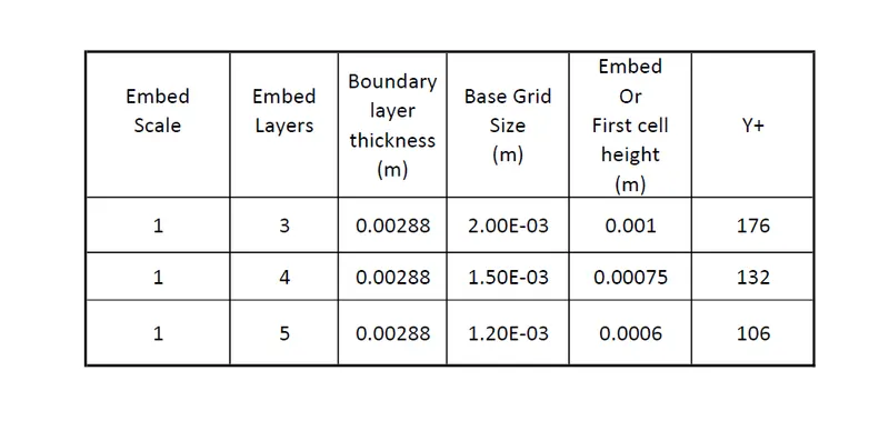
Keeping Embed scale to 1, for element size 2e−32e-3, the value of Embed is
Embed=0.0022Embed=0.0022
Embed=0.001mEmbed=0.001m
First cell height =0.001m=0.001m
While dealing with the control volume, y+y+ deals with the first cell centroid from the wall. The first cell height and the first cell centroid can be mathematically expressed as
△y=2yp△y=2yp
Therefore,
yp=0.0012yp=0.0012
yp=0.0005myp=0.0005m
y+=ρ∗Ut∗ypμy+=ρ∗Ut∗ypμ
y+=176.26=176y+=176.26=176
For element size 1.5e−31.5e-3, y+=132.19y+=132.19
For element size 1.2e−31.2e-3, y+=105.75y+=105.75
Summarising all values
Important commands used in Cygwin for post-processing the output files
The "cd" command is used for changing the directory. Once the command "cd" is utilized for navigating in the required directory. The simulation is performed by converging executable file, using a parallel processor (2) by using mpiexec.exe which is mpiexec.exe -n 2 "C:ProgramFilesConvergent_ScienceCONVERGE3.0.16binintelmpiconverge.exe" restricted </dev/null> logfile &.
The ampersand is used for dumping the output file into the log file.
In order to print the last ten lines of the output file "tail" command is used
tail -10 logfile.
The output folder contains the files which need to be post-converted by using post_convert_30_msmpi_64 which creates a .vtm group of files that is used for post-processing the results in "Paraview"
cd output
mpiexec.exe -n 2 post_convert_30_msmpi_64
Post-processing
The command used in "Cygwin" generates the ".vtm" group of files in the output folder, and the "Paraview" utilizes those groups of files to generate the results. The ".vtm" group of files is opened and the slice is made. The Z-normal is selected, the "Triangulate" option is checked off, "Show plane" is checked off. The "Surface with edges" is selected from the "Paraview" ribbon to visualize the mesh. The velocity magnitude contour plot and pressure contour plot are created and their respective animations were saved.
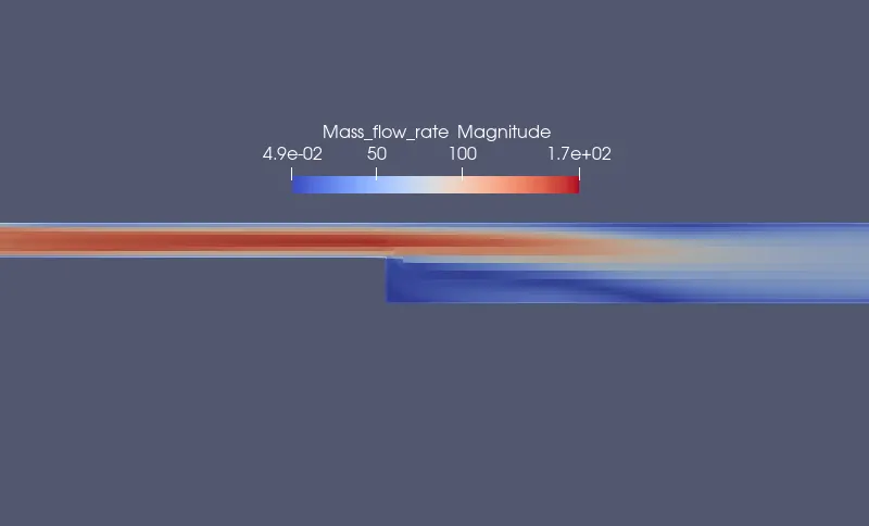
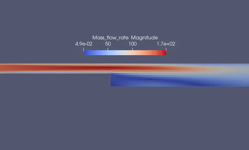
The "Mass flow rate magnitude" is a secondary variable and is dependent upon density and velocity which is further calculated by using the "calculator" option present in the "Filter" ribbon.
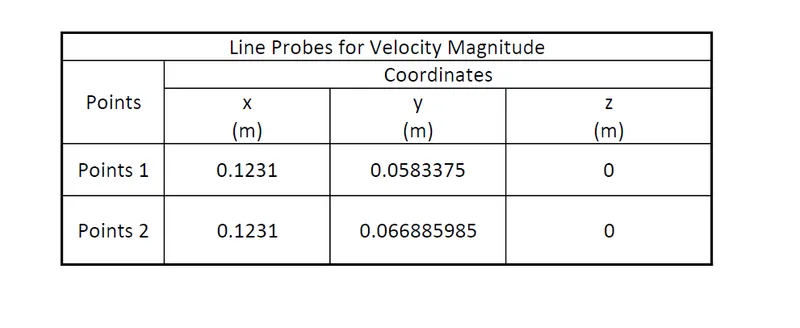
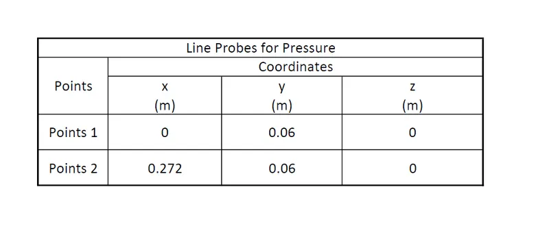
The "Plot over line" tool was selected from the ribbon and their variations were observed with the distances along with the domain.
Line-probes
Results
Mesh-1
Mesh-2
Mesh-3
Mesh-1
Contour plots
Velocity
Pressure
Mass flow rate
Animation file
Velocity
Pressure
Mass flow rate
Mesh-1
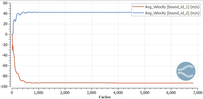
Velocity
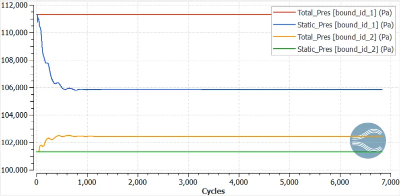
Pressure
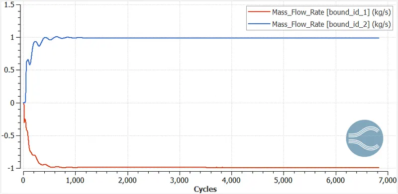
Mass flow rate
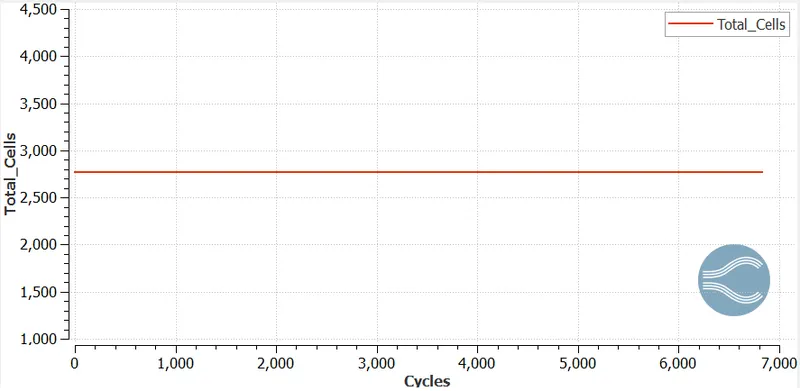
Total cells
Mesh-2
Velocity
Pressure
Mass flow rate
Animation file
Velocity
Pressure
Mass flow rate
Mesh-2
Velocity
Pressure
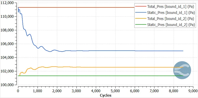
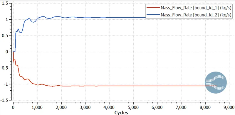
Mass flow rate
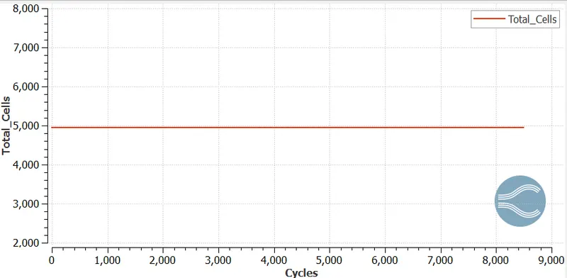
Total cell count
Mesh-3
Contour plots
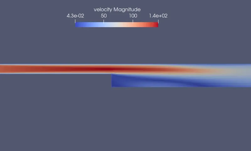
Velocity
Pressure
Mass flow rate
Animation file
Velocity
Pressure
Mass flow rate
Mesh-3
Velocity
Pressure
Mass flow rate
Total cells
Velocity plots for different mesh sizes
Pressure plots for different mesh sizes
Separation region
Mesh-3
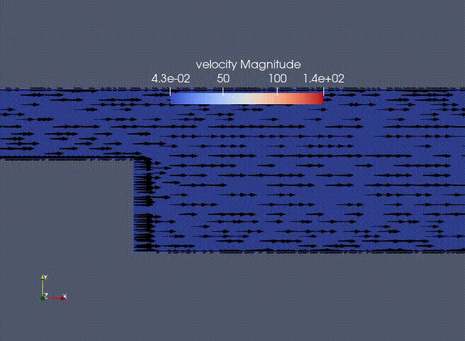
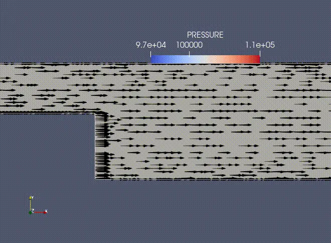
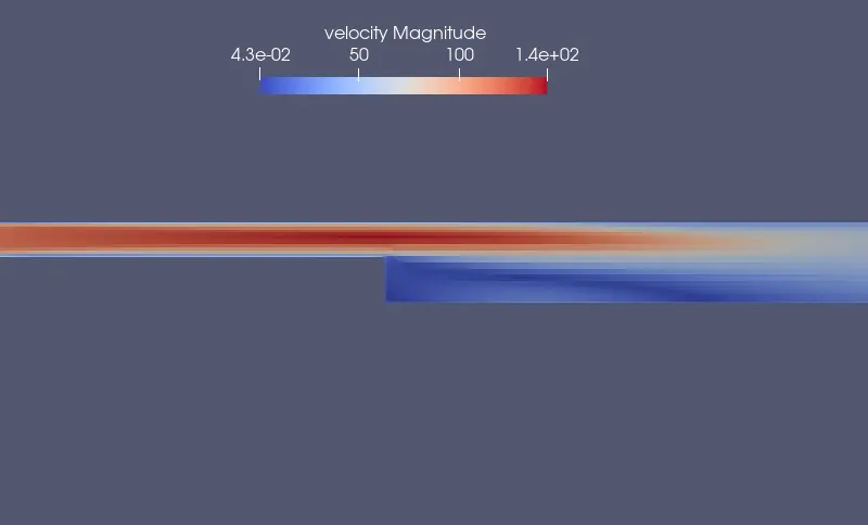
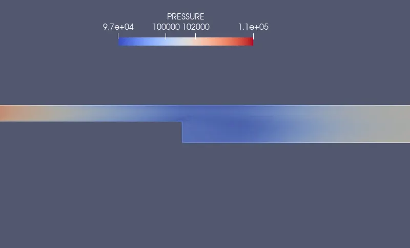
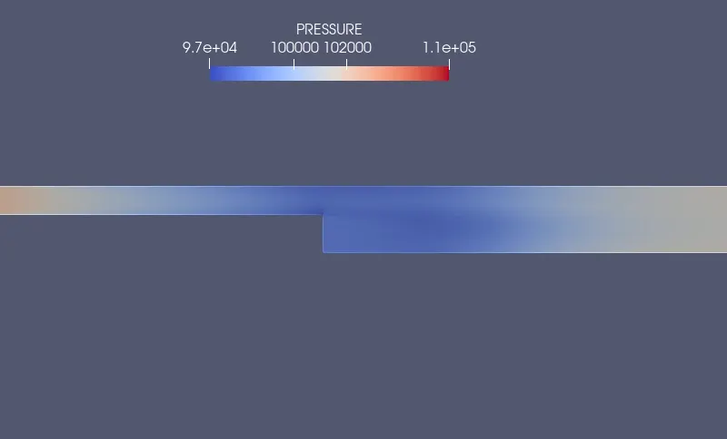
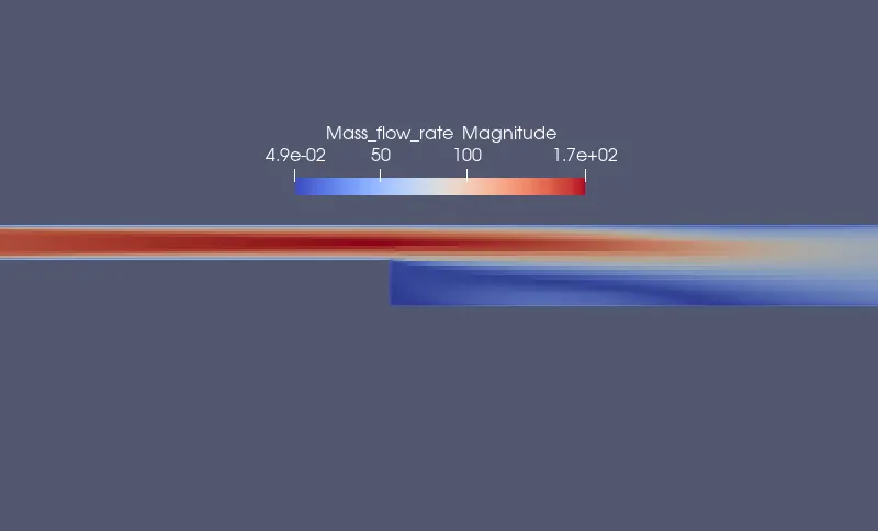
Air enters the inlet of backward-facing, due to the sudden changes in the geometry section at 0.1231m from the inlet, the air gets separated from the boundary leading to the deacceleration of the flow and reduction in the static pressure in that region, and beyond that, as seen in the above graphics file there are recirculation zones being formed and reattachment to the boundary layer occurs.
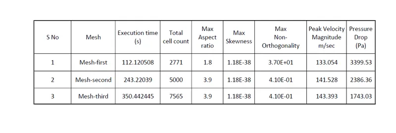
Comparison of all cases
Conclusion
- The steady-state simulation of the backward-facing step was carried successfully using the "Converge-CFD" and "Cygwin" command prompt terminal.
- As air enters the inlet of the backwards-facing step experiences turbulent flow, the turbulent flow is characterised by choosing the proper turbulence model to visualise the flow.
- The Realisable k−εk-ε model was chosen from the case setup tree and the default values were set accordingly.
- The turbulent flow initializes the formation of eddies near the wall and away from it. The size of the eddies are restricted near the wall and as we move away from the wall the size gets bigger. The flow is visualised in turbulent or log law region by choosing Y+ in the range of 30-300.
- The flow gets separated from the boundary layer after the step due to a change in the geometry and after the step, there are a recirculation zone and reattachment zones leading to the deacceleration of the fluid and thus reduction in the static pressure.
- The approximate value of Reynolds number leading to the determination of Y+, skin friction coefficient, frictional velocity was detrimental in the mesh refinement approach which included adding embed layers to the wall.
- The compressibility effect was observed in the flow leading to a Mach number greater than 0.3.
Source :
Generalized Cubic Equation of state [https://www.sciencedirect.com/topics/chemistry/cubic-equation-of-state]
Engineering Toolbox [https://www.engineeringtoolbox.com/]
Redlich Kwong Equation of state [https://en.wikipedia.org/wiki/Redlich%E2%80%93Kwong_equation_of_state]
Air-Thermophysical properties[https://www.engineeringtoolbox.com/air-properties-d_156.html#:~:text=Critical%20temperature%3A%20132.63%20K%20%3D%20%2D,3%20%3D%2018.89%20lbm%2Fft]
Embedding in Converge [https://skill-lync.com/knowledgebase/embedding-in-converge-2]
Fluid Mechanics Fundamentals and Applications- Yunus A. Cengel, John M. Cimbala